Global Mapper User's Manual
Download Offline Copy
If
you would like to have access to the Global Mapper manual while working
offline, click here to download the manual
web pages to your local hard drive. To use the manual offline, unzip the
downloaded file, then double-click on the Help_Main.html file from Windows
Explorer to start using the manual. If you would like context-sensitive help
from Global Mapper to use the help files that you have downloaded rather than
the online user's manual, create a Help subdirectory under the directory in
which you installed Global Mapper (by default this will be something like
C:\Program Files\GlobalMapperXX, where 'Program Files' could also be
'Program
Files (x86)' for a 32-bit install on 64-bit Windows and XX is the version, like
13 or 14. If you are running the 64-bit version this could also be
GlobalMapperXX_64bit) and unzip the contents of the zip file to that directory.
Open Printable/Searchable Copy (PDF Format) Table of Contents
1. ABOUT THIS MANUAL
a. System Requirements
b. Download and Installation
c. Registration
2. TUTORIALS AND REFERENCE GUIDES
♦ Tutorial -
Getting Started with Global Mapper and
cGPSMapper - Guide to Creating
Garmin-format
Maps
♦ Video
Tutorials - Supplied by http://globalmapperforum.com
◊ Video
Tutorial - Changing the Coordinate System and Exporting
Data
◊ Video
Tutorial - Viewing 3D Vector Data
◊ Video
Tutorial - Creating a Custom 3D Map
◊ Video
Tutorial - Downloading Free Maps/Imagery from Online
Sources
◊ Video
Tutorial - Exporting Current "Zoom Level" Using
the Screenshot Function
◊ Video
Tutorial - Exporting Elevation Data to a XYZ File
◊ Video
Tutorial - Creating Maps and Overlays for Google Earth
◊ Video
Tutorial - Georectifying Imagery/PDF Files 101
◊ Video
Tutorial - Importing ASCII files into Global Mapper
◊ Video
Tutorial - Exporting to Google Maps
◊ Video
Tutorial - Creating Range Rings, Importing Title Blocks,
and Address
Searching
◊ Video
Tutorial Creating Line from Selected
Points and Finding Max Slope Along
Path
♦ User-Supplied
Tutorials
◊ User-Supplied
Tutorial (from EDGAR) - How to Create 3D
Shadowed Maps
◊ User-Supplied
Tutorial - Garmin
Custom Raster Maps with Global Mapper
♦ Reference
Guide - Generic ASCII Format
♦ Reference
Guide - Generic ASCII Format Field Descriptions
♦ Reference
Guide - Shortcut Key Reference
♦ Reference
Guide - Supported Datum and Ellipsoid List
♦ Reference
Guide - Built-In Area, Line, and Point Types
and Styles
3. MENUBAR
AND TOOLBAR
a. File Menu
Open Printable/Searchable Copy (PDF Format) 1
• Open Data File(s) Command
• Open Spatial Database Command
• Open Generic ASCII Text File(s) Command
• Open All Files in a Directory Tree
• Open Data File at Fixed Screen Location
• Unload All Command
• Download Online Imagery/Topo/Terrain Maps
• Create New Map Catalog Command
• Rectify (Georeference) Imagery Command
• Load Workspace Command
• Save Workspace Command
• Save Workspace As Command
• Run Script Command
• Capture Screen Contents to Image Command
• Export Command
⋅ Export Global Mapper Package File
⋅ Export PDF File
⋅ Export Elevation Grid Format
⋅ Export Raster/Imagery Format
⋅ Export Vector Format
⋅ Export Web Formats (Google Maps, VE, WW, etc.)
⋅ Export Elevation Spatial Database Command
⋅ Export Raster/Image Spatial Database Command
⋅ Export Vector Spatial Database Command
• Batch Convert/Reproject
• Print Command
• Print Preview Command
• Print Setup Command
• Exit Command
b. Edit Menu
◊ Copy Selected Features to Clipboard
◊ Cut Selected Features to Clipboard
◊ Paste Features from Clipboard
◊ Paste Features from Clipboard (Keep Copy)
◊ Select All Features with Digitizer Tool
c. View
Menu
◊ Toolbars
◊ Status Bar
◊ 3D View
◊ Background Color
◊ Center on Location
◊ Properties
◊ Full View
◊ Zoom In
◊ Zoom In Micro
◊ Zoom Out
◊ Zoom Out Micro
◊ Zoom To Scale
◊ Zoom To Selected Features
◊ Zoom To View in Google Earth
◊ Save Current View
◊ Restore Last Saved View
d. Tools
Menu
◊ Zoom
◊ Pan (Grab-and-Drag)
◊ Measure
◊ Feature Info
◊ Path Profile/LOS (Line of Sight)
◊ View Shed Analysis
◊ Digitizer/Edit
⋅ Creating New Features
⋅ Editing Existing Features
⋅ Copying Features (Cut/Copy/Paste)
⋅ Snapping to Existing Features When Drawing
⋅ Snapping Vertically/Horizontally When Drawing
⋅ Un-doing Digitization Operations
⋅ Additional Feature Operations
◊ Image Swipe
◊ Coordinate Convertor
◊ Control Center
◊ Configure
◊ Map Layout
e. Terrain
Analysis Menu
◊ Combine Terrain Layers
◊ Generate Contours Command
◊ Generate Watershed Command
◊ Find Ridge Lines Command
◊ Measure Volume Between Surfaces Command
f. Search
Menu
g. GPS Menu
◊ Start Tracking GPS
◊ Stop Tracking GPS
◊ Keep the Vessel On-Screen
◊ Mark Waypoint
◊ Vessel Color
◊ Vessel Size
◊ Setup...
◊ Information...
◊ Manage GPS Vessels...
◊ View NMEA Data Log...
◊ Clear Tracklog
◊ Record Tracklog
◊ Save Tracklog
◊ Send Raster Maps to Connected Garmin Device
h. Help
Menu
◊ Online Help
◊ User's Group
◊ Find Data Online Command
◊ Register Global Mapper
◊ Create
S-63 User Permit File
◊ Check for Updates
◊ Automatically Check for Updates at Startup
◊ About Global Mapper
4.
OVERLAY CONTROL CENTER
a. Currently Opened Overlays
b. Metadata
c. Options
◊ Vector Data Options
◊ Raster Data Options
◊ Elevation Data Options
d. Show/Hide
Overlay(s)
e. Close Overlay(s)
5. LOADING FILES
a. Loading Multiple Files
b. Projections and Datums
6. CHANGE DISPLAY CHARACTERISTICS
a. General Options
b. Vector Display Options
c. Area Styles
d. Line Styles e. Point Styles
f. Vertical Options g. Shader Options
h. Projection Options
ABOUT THIS MANUAL
This
manual is for Global Mapper v14.0. Earlier versions of the software may not
contain all the features documented here. Later versions may contain additional
features, or behave differently. To see the version of your software, select
[Help/About Global Mapper] from the Menu Bar. The demo version contains some
but not all of the features available through a registered version of Global
Mapper.
The
Global Mapper Web Site found at: http://www.globalmapper.com maintains a list of changes and supported formats,
features, links to sample data as well as current information about the Global
Mapper software. Please refer to this site to obtain the latest copy of the
software.
Earlier versions of the software should be uninstalled
[Start/Settings/Control Panel/Add, Remove Programs]
before
installing later versions. System Requirements
Global
Mapper software is compatible with Windows 98, Windows NT, Windows 2000,
Windows ME, Windows XP (32 and 64-bit versions), Windows Vista (32 and 64-bit
versions), Windows 7 (32 and 64-bit versions), Windows 8 (32 and 64-bit
versions) and Windows Server 2003. You may also be able to run Global Mapper on
a Macintosh computer using an emulator like VirtualPC, Parallels, or Boot Camp,
or on a Linux
OS
under WINE. The minimum system requirements are 128 MB of RAM and 60 MB of hard
drive space for the installation. Space requirements for the data are typically
higher depending upon the size of the dataset.
Download
Step 1: Download the Global Mapper software
(latest version) from the Global Mapper website:
http://www.globalmapper.com by following the Download Free Trial link on the main page.
Step 2: Go to the directory in which you
saved the viewer in Step 1 and select the global_mapper14_setup.exe icon
Step 3: Double click the icon. Select
"YES" to install the program. Allow the installation to progress
normally and select any defaults it asked for.
Registration
You can freely download the latest version of Global Mapper
by following the instructions above. However, without a valid license, several
significant functions will be unavailable. In particular, if you do not obtain
a valid license for your copy of Global Mapper you will be subject to the
following limitations:
• You will
be unable to export data to any format.
• You will
be limited to loading a maximum of 4 data files at a time. With the full
version, you can load
any number of data files
simultaneously.
• You will
be unable to view loaded elevation data in 3D.
• You will
be unable to load workspaces.
• You will
be unable to do line of sight calculations using loaded elevation data.
• You will
be unable to perform view shed analysis using loaded elevation data.
• You will
be unable to perform cut-and-fill volume calculations using loaded elevation
data.
• You will
be unable to work with map catalogs.
• You will
be unable to download data from WMS, OSM, and TMS map servers.
• You will
be unable to save rectified imagery to fully rectified files.
• You will
be unable to join attribute files to loaded spatial data.
• You will
not be able to print to a specific scale (i.e. 1:1000).
• You will
have to endure a nagging registration dialog everytime that you run the
program.
• You will not
be eligible for free email support.
CLICK HERE TO REGISTER your copy of Global Mapper and obtain access to all of its
powerful features,
2 MENUBAR AND TOOLBAR
This section briefly reviews the
menus and commands in order to understand the basic purpose of each.
The toolbar is displayed across the top of the application
window, below the menu bar. The toolbar provides quick mouse access to many
tools used in Global Mapper. To hide or display the toolbars or to switch to
the old Toolbar display, which some users prefer, use the View menu commands
for the toolbar.
Menu Headings
• File Menu
• Edit Menu
• View Menu
• Tools Menu
• Search Menu
• GPS Menu
• Help Menu
File Menu
The File menu offers the following commands:
• Open Data File(s) Command
• Open Spatial Database Command
• Open Generic ASCII Text File(s) Command
• Open All Files in a Directory Tree Command
• Open Data File at Fixed Screen Location
• Unload All Command
• Create New Map Catalog Command
• Find Data Online Command
• Download Online Imagery/Topo/Terrain Maps
• Load Workspace Command
• Save Workspace Command
• Save Workspace As Command
• Run Script Command
• Capture Screen Contents to Image Command
• Export
Submenu
♦ Export Global Mapper Package File Command
♦ Export PDF File Command
♦ Export
Gridded Elevation Data
◊ Export Arc ASCII Grid Command
◊ Export BIL/BIP/BSQ Command
◊ Export BT (Binary Terrain) Command
◊ Export DEM Command
◊ Export DTED Command
◊ Export DXF 3D Face File Command
◊ Export DXF Mesh Command
◊ Export DXF Point File Command
◊ Export Erdas Imagine Command
◊ Export ERS (ERMapper Grid) Command
◊ Export Float/Grid Command
◊ Export Geosoft Grid Command
◊ Export GeoTIFF Command
◊ Export Global Mapper Grid Command
◊ Export Gravsoft Grid Command
◊ Export HF2/HFZ Command
◊ Export Idrisi Command
◊ Export JPEG2000 Elevation Command
◊ Export Lidar LAS Command
◊ Export Lidar LAZ (Compressed LAS) Command
◊ Export Leveller Heightfield Command
◊ Export Optimi
Terrain Command
◊ Export PGM
Grayscale Grid Command
◊ Export PLS-CADD
XYZ File Command
◊ Export RAW Command
◊ Export RockWorks Grid Command
◊ Export SRTM Command
◊ Export STL Command
◊ Export Surfer Grid (ASCII Format) Command
◊ Export Surfer Grid (Binary v6 Format) Command
◊ Export Surfer Grid (Binary v7 Format) Command
◊ Export Terragen Terrain File Command
◊ Export Vertical Mapper (MapInfo) Grid File Command
◊ Export Vulcan3D Triangulation File Command
◊ Export XYZ Grid Command
◊ Export ZMap Plus
Grid File Command
♦ Export Raster/Imagery Format
◊ Export BIL/BIP/BSQ
Command
◊ Export BMP
Command
◊ Export BSB
Marine Chart Command
◊ Export
CADRG/CIB/RPF Command
◊ Export ECW
Command
◊ Export Erdas
Imagine Command
◊ Export GeoTIFF
Command
◊ Export Idrisi
Command
◊ Export JPG
Command
◊ Export JPG2000
Command
◊ Export KML/KMZ
Command
◊ Export NITF
Command
◊ Export PCX
Command
◊ Export PNG Command
◊ Export RAW Command
◊ Export XY Color Command
♦ Export
Vector Format
◊ Export AnuDEM Contour Command
◊ Export Arc Ungenerate Command
◊ Export CDF Command
◊ Export CSV Command
◊ Export Delft 3D (LDB) Command
◊ Export DeLorme
Text File Command
◊ Export DGN
Command
◊ Export DLG-O
Command
◊ Export DXF
Command
◊ Export DWG
Command
◊ Export Esri File
Geodatabase Table Command
◊ Export Esri
Personal Geodatabase Table Command
◊ Export Garmin
TRK (PCX5) File Command
◊ Export Garmin
WPT (PCX5) File Command
◊ Export GeoJSON (Javascript Object Notation) Command
◊ Export GOG (Generalized Overlay Graphics) Command
◊ Export GPX Command
◊ Export Hypack Linefile
◊ Export InRoads ASCII Command
◊ Export KML/KMZ Command
◊ Export Landmark Graphics Command
◊ Export Lidar LAS Command
◊ Export Lidar LAZ (Compressed LAS) Command
◊ Export LMN (Spectra Line Management Node) Command
◊ Export Lowrance LCM (MapCreate) File Command
◊ Export Lowrance USR Command
◊ Export MapGen Command
◊ Export MapInfo MIF/MID Command
◊ Export MapInfo TAB/MAP Command
◊ Export MatLab Command
◊ Export Moss Command
◊ Export NIMA ASC Command
◊ Export Orca XML Command
◊ Export OSM (OpenStreetMap.org) XML Command
◊ Export Platte River/WhiteStar/Geographix File Command
◊ Export PLS-CADD XYZ File Command
◊ Export Polish MP (cGPSMapper) File Command
◊ Export SEGP1 Command
◊ Export Shapefile Command
◊ Export Simple ASCII Text File Command
◊ Export Surfer BLN Command
◊ Export SVG Command
◊ Export Tom Tom OV2 File Command
◊ Export Tsunami OVR Command
◊ Export UKOOA P/190 Command
◊ Export WAsP MAP File Command
◊ Export ZMap+ IsoMap Line Text File Command
◊ Export ZMap+ XYSegId File Command
♦ Export Web
Formats (Google Maps, VE, WW, etc.)
◊ Export Bing Maps (Virtual Earth) Tiles Command
◊ Export Google Maps Tiles Command
◊ Export KML/KMZ Command
◊ Export OSM (OpenStreetMaps.org) Tiles Command
◊ Export SVG Command
◊ Export TMS (Tile Map Service) Tiles Command
◊ Export VRML Command
◊ Export World Wind Tiles Command
◊ Export Zoomify Tiles Command
♦ Export Elevation Spatial Database Command
♦ Export Raster/Image Spatial Database Command
♦ Export Vector Spatial Database Command
♦ Batch Convert/Reproject
• Print Command
• Print Preview Command
• Print Setup Command
• Exit Command
Open Data File(s) Command

The
Open Data File(s) command allows the user to open additional data files into
the main Global Mapper view. If no other data is already loaded and the user
has not explicitly set a projection, the view will adopt the projection and
datum of the first data file selected for loading. If other data is already
loaded, the selected data files will be displayed in the current
projection/datum.
The
data will automatically be displayed at the proper location relative to other
loaded data, creating a mosaic of data that is properly placed spatially. You
don't have to do anything special to create mosaics of multiple files, this
happens simply by loading the geo-referenced files into Global Mapper.
Note:
Global Mapper automatically opens files with tar.gz extensions without the use
of a decompression tool such as Winzip. This is particularly useful for SDTS
transfers, which are typically distributed in a .tar.gz format.
The
Open Spatial Database command allows the user to open additional data into the
main Global Mapper view from a spatial database connection. If no other data is
already loaded and the user has not explicitly set a projection, the view will
adopt the projection and datum of the first spatial table selected for loading.
If other data is already loaded, the selected data files will be displayed in
the current projection/datum.
Click here for more information about loading data from a spatial
database. Open Generic ASCII Text File(s) Command
The Open Generic ASCII Text File(s) command allows the user
to import data from a wide variety of generic
ASCII text formats.
Selecting
the Open Generic ASCII Text File command prompts the user to select the file(s)
to load and then displays the Generic
ASCII Text Import Options dialog (pictured below). This dialog allows the
user to specify how the text file(s) are formatted so that they can be
imported.
Global
Mapper supports coordinates in decimal format as well as degree/minute and
degree/minute/second coordinates.

The
Import Type section allows the user
to specify how they want the data in the file to be treated. The different
import types are defined as follows:
• Point Only - All lines from the file which are
determined to contain coordinate data will result in a
single point feature to be
generated.
• Point, Line, and Area Features - Any
string of two or more consecutive lines with coordinate data
will result in a line or area
feature. All isolated coordinate lines will result in a point feature.
• Elevation Grid - All lines from the file
which are determined to contain 3D coordinate data will be
use generated a triangulated terrain
which is then gridded to create a elevation grid. This grid has all
the capabilities of an imported DEM, including contour
generation, line of sight and view shed analysis, and raster draping. When
selecting this option, the Create Elevation Grid dialog will appear
after setting up the ASCII file import options to allow setting up the gridding
process.
The
Coordinate Column Order section
allows the user to specify in what order the coordinates are found on
coordinate lines in the file. Coordinates can either be x followed by y (i.e.
longitude then latitude) or the reverse. You can also load files with WKT
(well-known-text) coordinate strings, allowing line, polygon, and point feature
coordinates all on a single line. MGRS (military grid reference system) coordinate
strings can also be loaded. Elevation values, if any, are always assumed to
come after the x and y values.
The
Fields to Skip at Start of Line setting
controls what field index (column) the coordinates start in. For example, if
the x and y coordinates are in the 3rd and 4th columns, set this value to 2 so
that the coordinates will be grabbed from the appropriate place. The Coordinate Format option allows you to
specify how coordinate values are stored. The default option supports several
formats, including using the exact decimal representation for the coordinate
and automatic recognition of separated latitude/longitude degree values, such
as DD MM SS with a large variety of supported separating characters. Support
also exists for packed decimal
degree values in the formats DDMMSS.S and DDMM.M.
The
Coordinate Delimeter section allows
the user to specify what character the coordinates are separated by on
coordinate lines. If the Auto-Detect option
is selected, Global Mapper will attempt to automatically determine the
coordinate delimeter. This option will usually work and should probably be used
unless you have trouble.
The
Coordinate Line Prefix section allows
the user to specify whether coordinates start at the beginning of the line or
if coordinate lines start with some other sequence of characters. For example,
some formats may start coordinate lines with the sequence "XY,".
The
Rows to Skip at Start of File setting
controls how many lines to skip at the start of the file before trying to
extract data. This is useful if you have some header lines at the start of your
file that you want to skip over.
The
Feature Classification section allows
the user to specify what feature type to assign to area, line, and point
features imported from the file.
If
the Include attributes from lines with
coordinate data option is selected, any text found AFTER the coordinate
data on a line from the file will be including as attribute for the feature
that coordinate is in. If not selected, only lines from the file that are not
determined to contain coordinate data will be used as attributes.
If you are doing a Point Only import and the Column Headers in First Row of File option
is checked, values
in
the first line from the file will be used at the names of attributes for
attributes found in coordinate data lines. This is useful for things like CSV
files.
If
the Treat 3rd coordinate value as
elevation option is selected and a numeric value is found immediately
following the x and y (or lat and lon) coordinate values, that value will be
treated as an elevation. Otherwise, the value will be included as an attribute
if the Include attributes from lines with
coordinate data option is selected. Typically you want to leave this option
checked unless you are importing point data in which the 3rd column is an
attribute that occasionally contains all numeric values, such as well names.
If
you have line and/or area data that do not have non-coordinate lines separating
them but rather are delimited by a change in a particular field/column of data,
you can use the Break Line/Area Features
on Change in
Field option
to specify which field (use a 1-based index) to check for breaking the data
into separate line/area features.
Pressing
the Select Coordinate Offset/Scale button
displays a dialog that allows the user to select an offset and scale factor to
apply to each coordinate. The offset entered will first be added to each
coordinate, and then
each coordinate will be multiplied by the scale factor.
When
generic ASCII text files are imported, Global Mapper will scan the attributes
associated with each feature and look for any attribute names that are known to
it. The following is an abbreviated list of attribute names that are currently
recognized by Global Mapper when generic ASCII text files are read (see the
links below the list for more complete lists):
• NAME or
LABEL - the value associated with an attribute of either of these names will be
used as the
feature name.
• DESC,
DESCRIPTION, LAYER, or TYPE - the value associated with an attribute of any of
these
names will be used as the feature
description.
• GM_TYPE -
the value associated with an attribute with this name or any of the description
names
listed above will be used to attempt
to assign a classification other than the default for each feature.
The value must match one of the classification names in
Global Mapper to work. It will also work for user-created custom types.
• ELEVATION,
HEIGHT, or DEPTH - the value associated with an attribute of any of these names
will be used as the feature's
elevation.
• SYMBOL,
POINT SYMBOL, or POINT_SYMBOL - the values associated with an attribute of any
of these names will be compared
against the names of the symbols available in Global Mapper
(including any custom symbols). If a match is found, that
symbol will be used for the point feature. These attribute names are ignored
for line features. You can also specify custom dot and square symbol colors and
sizes without having to add your own custom bitmaps for those symbols. Use
names of the form DOT_CUSTOM_[SIZE]_[RED]_[GREEN]_[BLUE] and
SQUARE_CUSTOM_[SIZE]_[RED]_[GREEN]_[BLUE] where the [SIZE] value is the radius
in pixels of the dot or square, and the [RED], [GREEN], and [BLUE] values
represent the color to use. For example, to specify a dot symbol of radius 10
pixels with a color or green, you would use a symbol name of
DOT_CUSTOM_10_0_255_0.
• COLOR -
the COLOR attribute should be formatted as RGB(red,green,blue). In the absence
of a
specific fill or line color, it will
be used.
• LINE
COLOR, LINE_COLOR, BORDER COLOR, BORDER_COLOR, PEN COLOR, or
PEN_COLOR - the values associated
with an attribute of any of these names will be used as the color
for the pen used to draw line features. The values must be
formatted according to the guidelines layed out for the COLOR attribute in
order to be recognized.
• LINE
WIDTH, LINE_WIDTH, BORDER WIDTH, BORDER_WIDTH, PEN WIDTH, or
PEN_WIDTH - the values associated
with an attribute of any of these names will be used as the width
for the pen used to draw line features.
• LINE
STYLE, LINE_STYLE, BORDER STYLE, BORDER_STYLE, PEN STYLE, or PEN_STYLE
- the values associated with an
attribute of any of these names will be used as the style for the pen
used to draw line features. Valid values are Solid, Dash,
Dot, Dash - Dot, Dash - Dot - Dot, and Null. Only the Solid value is valid for
lines with a width greater than 1
• LABEL_ON_LINE
- if this is set to "YES" or "TRUE", the label (if any) for
this line feature should
be rendered centered on the line
• CLOSED -
if this is set to "YES" or "TRUE", the feature will be
treated as a closed area feature if it
has at least three vertices.
• ISLAND -
if this is set to "YES" or "TRUE", the feature will be
treated as an island of the previous
closed parent area feature if it has
at least three vertices. If there are no previous parent areas, this
attribute will be ignored.
• FONT_NAME
- specifies the name (e.g. Arial, Times New Roman, etc.) of the font to use
when
displaying the display label, if
any, for this feature.
• FONT_COLOR
- specifies the color of the font to use when displaying the display label, if
any, for
this feature. The values must be
formatted according to the guidelines layed out for the COLOR
attribute in order to be recognized.
• FONT_ANGLE
- specifies the angle in degrees of the font to use when displaying the display
label, if
any, for this point feature.
• FONT_SIZE
- specifies the point size of the font to use when displaying the display
label, if any, for
this feature.
• FONT_HEIGHT_METERS
- specifies the height in meters of the font to use when displaying the
display label, if any, for this
feature. Using this causes the actual point size of the font to vary as you
zoom in and out.
• FONT_CHARSET
- specifies the numeric character set of the font to use when displaying the
display
label, if any, for this feature.
These correspond to the Windows character set enumeration.
Click here for more instructions on creating generic ASCII data files with features of
various types and click here for more documentation on the supported
fields.
 Download Online Imagery/Topo/Terrain Maps
The
Download Online Imagery/Topo/Terrain Maps command allows the user to download
mapping data from numerous built-in and user-supplied sources. This includes
premium access to high resolution color imagery for the entire world from DigitalGlobe, worldwide street maps from OpenStreetMap.org, as well as seamless USGS topographic maps and satellite
imagery for the entire United States from
MSRMaps.com/TerraServer-USA.
In addition, access is provided to several built-in WMS (OpenGC Web Map Server)
databases to provide easy access to digitial terrain data (NED and SRTM) as
well as color satellite imagery (Landsat7) for the entire world. You can also
add your own WMS data sources for access to any data published on a WMS server.
This
is an extremely powerful feature as it puts many terabytes of usually very
expensive data right at your fingertips in Global Mapper for no additional cost
(with the exception of access to the un-watermarked DigitalGlobe imagery, which
is not free). Note that this feature requires Internet access to work.
When
you select the menu command, the Select
Online Data Source to Download dialog (pictured below) is displayed. This
dialog allows you to select the type, or theme, of data to download, as well as
the extents of the data to download. You can either select to download the
current screen bounds, an area to download around an address, specify a lat/lon bounds explicitly, or select to download
the entire data source.

Once
the data to download is defined, Global Mapper will automatically download the
most appropriate layer for display as you zoom in and out. This way, you can
see an overview of the data when zoomed out, with more detail becoming
available when you zoom in. You can also export this data in full resolution to
any of the supported raster export formats, such as GeoTIFF, JPG, or ECW. The
most appropriate detail level for the export sample spacing will be used to
obtain the source data for the export.
Each
data source load will appear as a separate layer in the Overlay Control Center.
Each entry can have it's display options modified just like any other raster
layer to drape it over elevation data, blend it with other layers, etc.
You
can use the Add New Source button to add new online sources of imagery from WMS
(Web Map Service), WCE (Web Coverage Service), OSM (OpenStreetMap Tiles),
Google Maps-organized tiles or TMS (Tile Map Service) sources. When you press
the button a dialog appears allowing you to choose the type of source to add.
If you select the WMS or WCS option then the Select WMS Data Source to Load dialog (pictured below) is
displayed. This dialog allows you to specify the URL of a WMS or WCS data
source and select what layer(s) to add as an available data source on the Select Online Data Source to Download dialog.
The URL that you should specify is the GetCapabilities URL, such as
http://wms.jpl.nasa.gov/wms.cgi for the JPL WMS data server. Once you've
entered the URL, press the Get List of Available Data Layers button to query
the server and populate the data control with the available data layers on that
server. Then simply select the data layer and style that you want and press OK
to have it added to the available data source list. Once a
source
is added, you can use the Remove Source button to remove it from the list of
available data sources at a later time. If you need to specify additional
options for the WMS server, such as forcing a particular image format to be
used, add those parameters after the Service Name parameter. For example, to force
the use of
the
JPG format, you might specify a Service Name parameter of
'WMS&format=image/jpeg'. To force a particular projection that the server
supports to be used, include a SRS parameter, like
'WMS&SRS=EPSG:26905' to force the use of the UTM projection
with the NAD83 datum and zone 5N.
You
can also right-click on the added WMS layer in the list of sources and set a
maximum zoom level (in meters per pixel) for the layer. For example you can
specify a maximum zoom level of 5.0 meters per pixel, so when loading data from
the source no tiles with a resolution greater than 5.0 meters per pixel will be
downloaded. This is useful for sources that don't specify themselves what the
maximum resolution should be and just go blank when you overzoom them.
You
can also right-click on the added WMS layer in the list of sources and check
whether or not to download as tiles when drawing or to download a single image
for each draw operation. The default is to use tiles as that allows caching so
that if you revisit an area at the same zoom level you don't have to redownload
it. However if you have a source that adds a watermark to each tile this may be
undesirable. Uncheck this option to disable the use of tiles for display. They
will still be used for export as the size of exports makes it impossible to
fetch all at once in many cases.

If
you choose the OSM, Google Maps, or TMS source type, then the OSM/TMS Tile Source Defintion dialog
(pictured below) is displayed, allowing you to setup the source. You need to
specify the base URL where the data for the tiled source can be found (this
should be the folder under which the folders for each zoom level are stored).
You can also provide a URL with variables named %x (column), %y (row), and %z
(zoom scale) in the URL so that you can setup the URL however your data source
requires rather than using the default expected URL setup. If accessing a
source setup similar to Bing Maps tiles, you might need to use the quadtree
filename. Use %quad to do this. This replaces the %x, %y, and %z values.
Finally the Bing Maps
RESTful
services supports accessing via the zoom scale (%z) and a latitude and
longitude value in the tile. Use %lat and %lon to include the latitude and
longitude of the center point of the tile in your custom URL. You also must
select whether the source uses PNG or JPG image files and provide the maximum
zoom level and bounds of the data source.

You
can also use the Delete Cached Files button to remove any locally cached files
from any particular type of data sources. This is useful if the online data may
have changed or if you have downloaded corrupt files somehow.
The
Add Sources From File button allows you to add new WMS sources from an external
text file. This provides an easy way to share your list of WMS sources with
other users. You can simply provide them with your wms_user_sources.txt file
from your Application Data folder (see the Help->About dialog for the
location of this folder) and they can load that file with this button to add
their sources to your source list.
The Load ECW from Web button allows the user to open an ER
Mapper Compressed Wavelet (ECW) image file directly from an Image Web Server
URL using the ECWP protocol. While these files may be terabytes in actual size,
only the portion needed for the current display window is downloaded, allowing
for the browsing of extremely large data sets.
Selecting
the Load ECW from Web displays the Load
Image From Web dialog (pictured below). This dialog allows the user to either
select a predefined web link for loading or to enter the URL of any available
ECW file served by Image Web Server.

The tree on the left of the dialog allows the user to select
which data file they wish to load. Global
Mapper
comes with several dozen useful links already entered into
the tree.
To access your own ECW image from the web, press the Add Link... button. This button causes
the Add New
Web Link dialog (pictured below) to be displayed.

The Group Name drop
list allows the user to select which group, if any, to place the new link in.
Any of the predefined groups can be selected, or a new group name can be
entered. Leaving the group name blank will cause the new link to appear at the
root level of the tree.
The
Description field is where you enter
the human-readable description of the link. This is what will be displayed for
the link on the main dialog. Leaving this blank will cause the URL to be
displayed instead.
The
URL field is the most important piece
of this dialog. This is where you specify the address of the ECW file to load.
The URL should begin with the prefix ecwp://
with the remainder being a valid path to an ECW file served using ER
Mapper's Image Web Server software.
When
you've completed entering information about the new web link, press the OK button to complete your entry and
have it added to the web link tree in the Load
Image From Web dialog.
Pressing
the Edit Link... button allows the
user to edit the currently selected web link. Note that the built-in web links
cannot be edited.
Pressing the Delete
Link... button will delete the currently selected web link or group from
the web link tree.
If you get an error message indicating that your settings
have been updated to support the ECWP protocol whenever you try to load an ECW
layer from the web you need to download and install the latest ECW ActiveX
plugin from http://demo.ermapper.com/ecwplugins/DownloadIEPlugin.htm.
Open All Files in a Directory Tree Command
The Open All Files in a Directory Tree command allows the
user to open all of the files matching a
user-specified
filename mask under a user-selected directory. You will first be prompted to
select a folder from which to load the files. After selecting the folder, you
will be prompted to enter a filename mask for all of the files that you would
like to attempt to load. After selecting a filename mask, all files under the
selected folder which match the filename mask and are recognized by Global
Mapper as a known data type will be loaded.
The
filename mask supports the * and ? wildcard characters. The default mask of *
will check all files under the selected folder. You can also cause data to only
be loaded from selected folders as well. For example, if you had a large
collection of folders with data split up into 1x1 degree blocks with the folder
names depecting the 1x1 degree block they held, you could use a directory name
mask to load only those blocks that you wanted. For example, you might use a
mask of N4?W10?\*.tif to load all
TIFF files between N40 and N50
and W110 and W100.
You
can also specify multiple masks if you need more than one to describe the set
of files that you would like to load. Simply separate the masks with a space.
Open Data File at Fixed Screen Location
The
Open Data File at Fixed Screen Location command allows the user to open any
supported data file format for display at a fixed location on the screen rather
than at a fixed location on the earth. This is particularly useful for loading
things like bitmaps for legends and logos. The loaded data will be used for
screen display, export, and printing operations.
Selecting
the Open Data File at Fixed Screen Location command first prompts you to select
a file to load, then displays the Fixed
Screen Location Setup dialog (pictured below). This dialog allows the user
to specify the size and position of the data relative to the
screen/export/printout.

Unload All Command
The
Unload All command unloads all overlays and clears the screen. Create New Map
Catalog Command
The
Create New Map Catalog command allows you to create a "map catalog".
A "map catalog" is a collection of map files which are grouped
together to allow for easy loading, viewing, and export. Layers in a map
catalog will be loaded and unloaded as needed for display and export,
potentially greatly reducing the load time and memory requirements for working
with very large collections of data.
Upon
selecting this command and selecting the file to save the map catalog to, the Modify Map Catalog dialog (shown below)
will be displayed, allowing you to add files to the catalog, control at what
zoom level data layers are loaded for display, and setup how the map bounding
boxes are displayed when you are zoomed out too far for the actual map data to
display. By default map bounding boxes are displayed using the style set for
the Map Catalog Layer Bounds type.

You
can obtain metadata and projection information about layers in the map catalog
by right-clicking on them in the Map List and selecting the appropriate option.
You
can modify map catalogs again after loading them by opening the Overlay Control Center, selecting the
map catalog layer, then pressing the Options button.
Note:
Only registered users of Global Mapper are able to create map catalogs. Load
Workspace Command
The
Load Workspace command allows the user to load a Global Mapper workspace file
(.gsw) previously saved with the Save Workspace
command.
Note:
Only registered users of Global Mapper are able to load Global Mapper workspace
files. Save Workspace Command
The
Save Workspace command allows the user to save their current set of loaded
overlays to a Global Mapper workspace file for later loading with the Load Workspace command.
The
Global Mapper workspace maintains the list of all currently loaded overlays as
well as some state information about each of those overlays. When the workspace
file is loaded, all of the overlays that were loaded at the time the workspace
file was saved will be loaded into Global Mapper. This provides a handy way to
easily load a group of overlays which you work with often.
The Global Mapper workspace will also contain any changes
that you have made to loaded vector features as well as any new vector features
that you have created. The user projection and last view on the data will also
be maintained.
Find Data Online Command
Selecting
the Find Data Online command will open a web browser pointing to places on the
internet where data compatible with Global Mapper is available for download.
Run Script Command
The
Run Script command allows users to run a Global Mapper script file that they
have created. This is a powerful option that allows the user to automate a wide
variety of tasks. Click here for a guide to
the scripting language.
Selecting the Run Script command from the menu displays the Script Processing dialog, shown here.

The Script File pane
displays the currently loaded script file. To load a new script file for
processing, press the
Load Script... button at the bottom left corner of the dialog.
If
you would like the script file to make use of data already loaded in the main
view and to also affect what is displayed in the main view, check the Run Script in the Context of the Main View option
prior to running the script.
To
run the loaded script file, press the Run
Script button. Any warning, error, or status messages generated while
running the script will be output to the Script
Results pane.
When you are done processing scripts, press the Cancel button to close the dialog.
Note:
Only registered users of Global Mapper are able to run Global Mapper script
files. Capture Screen Contents to Image Command
The
Capture Screen Contents to Image command allows user to save the current
contents of the Global Mapper window to a JPEG, PNG, (Geo)TIFF, or Windows
Bitmap (BMP) file. In addition, the generated image can be generated in a
higher resolution than the screen to provide greater fidelity. Also, a world
file for georeferencing in other software packages as well as a projection
(PRJ) file describing the native ground reference system of the image can be
optionally generated as well.
Unlike
the raster export commands described later, the Capture Screen Contents to
Image command also saves any vector overlays drawn to the screen.
Selecting the Capture Screen Contents to Image command from
the menu displays the Screen Capture
Options dialog,
shown here.

The
Image Format section allows the user
to select the format of the image to generate. Different formats have their own
unique strenghts and weaknesses which make choosing the best format vary
depending on the desired end results. The supported formats are:
• JPEG - JPEG is a lossy format that achieves excellent
compression on images with a lot of color
variation, such as pictures of real
world objects and shaded elevation data.
• PNG (Portable Network Graphic) - PNG is a
lossless format that achieves excellent compression on
images without a lot of color
variation, such as line (vector) drawings and paper map scans such as
DRGs. The generated PNG file will be of the 24-bit variety.
• (Geo)TIFF - TIFF is a lossless format that is supported
by many GIS packages. Saving the screen to a
TIFF with this command generated a
24-bit uncompressed TIFF. In addition, all georeferencing data
is stored in a GeoTIFF header attached to the TIFF, making
the image completely self-describing.
• Windows Bitmap (BMP) - BMP is a widely support
format on Windows platforms. Saving the screen
to a BMP results in a 24-bit
uncompressed image.
The
width and height of the generated image in pixels are specified in the Image Size panel. By default, the size
of the Global Mapper view pane are used. Using these values will generate an
image that exactly matches what you see. You can change these values to
generate a more or less resolute image with the obvious tradeoff of size vs.
quality.
Checking
the Generate World File option
results in a world file being generated in addition to the image. The world
file will be generated in the same directory as the image and will have the
same primary name as the image. The filename extension will depend on the
selected image type (JPEG=.jpgw, PNG=.pngw, TIFF=.tfw,BMP=.bmpw).
Checking
the Generate Projection (PRJ) File option
results in a projection file being generated describing the ground reference
system of the created image. The projection file will be generated in the same
directory as the image and will have the same primary name as the image with an
extension of .prj.
Checking
the Generate Text Metadata File option
results in a text file being generated listing the metadata for the captured image.
Checking
the Crop to Loaded Map Data option
results in a text file being generated that is cropped to the bounds of your
currently loaded map data rather than the full screen extents. If the loaded
map data does not take up at least the entire screen then your specified pixel
dimensions will also be shrunk so that the pixel size remains the same.
Pressing
the OK button prompts the user to
select the name and location of the image to generate and then proceeds to
generate the image.
Note:
Only registered users of Global Mapper are able capture the screen to an image
file. Export Global Mapper Package File Command
The
Export Global Mapper Package File command allows the user to export any or all
of the loaded data to a Global Mapper package file. These files are similar to
workspace files except that the actual data is stored in the files. Package
files provide an easy way to pass around lots of data between Global Mapper
users on different computers with a single self-contained file.
When
selected, the command displays the Global
Mapper Package Export Options dialog which allows the user to setup the
package export. The dialog consists of a Package
Options panel, a Simplification panel,
a Gridding panel, and an Export Bounds panel.

The
Package Options panel consists of
options allowing the user to select the projection to save the data in, how to
handle dynamically streamed MSRMaps.com/TerraServer-USA data, and other
options. These include the Always
Maintain Feature Styles option, which specifies that any vector features
stored in the package file should explicitly save the styling of that feature,
even if they are using the default style for the feature classification. This
can make it easier to maintain exact styling when transferring packages between
Global Mapper installations.
In
the Projection section of the panel,
the user can choose to save all loaded data in the currently selected view
projection (this is the projection selected on the Projection tab of the
Configuration dialog), in latitude/longitude coordinates (the
"Geographic" projection) with the WGS84 datum, or to keep each layer
in its original native projection.
In
the TerraServer Export Options section
of the panel, the user can select how displayed layers from the Download
TerraServer menu option are exported. The Automatic
selection for imagery themes (i.e. DOQs, Urban Area imagery) will save data
slightly more detailed than what is displayed on the screen. For the DRG
(topographic map) theme, the most detailed zoom range for the current scale of
DRG map being displayed
(i.e. 24K, 100K, 250K) will be determined and data from that
scale will be saved. The other alternatives either
save
the most detailed scale available, creating potentially very large files, or
the scale the most closely matches the current display scale on the screen.
The
Combine Compatible Vector Layers into a
Single Layer option causes all vector features with the same native
projection to be combined into a single layer within the package file rather
than maintaining their original layer structure.
The Embed Images
Associated with Picture Points option causes any images associated with a
vector feature
(like points from an EXIF JPEG file) to be embedded in the
GMP file for easy use on other systems.
The
Simplification panel allows the user
to set up the threshold at which points that don't contribute much to the shape
of the vector line and area features being exported are removed in order to
generate features with less vertices. By default, all vertices will be kept,
but the user can move the slider to the right to get rid of relatively
insignificant vertices and realize significant space spacings at the cost of
some fidelity.
The
Gridding panel allows the user to split up
the data into regularly spaced tiles on export if desired rather than just
exporting a single file.
The
Export Bounds panel allows the user to
select what portion of the loaded data they wish to export. Note: Only registered users of Global Mapper
are able capture the screen to an image file.
Export PDF/GeoPDF File Command
The
Export PDF File command allows the user to export any or all of the loaded data
to a Geo-enabled PDF file. These are standard PDF files that can be read in
Adobe Acrobat Reader. They also will have geopositioning information embedded
in them so that mapping applications like Global Mapper can automatically
display the data in the PDF at the proper location.
When selected, the command displays the PDF Export Options dialog which allows the user to setup the PDF
export. The dialog consists of a PDF Options panel, a Gridding
panel, and an Export Bounds panel.

The
PDF Options tab allows the user to
setup the PDF-specific export options. The following sections are available:
• Page Setup
♦ Page Size - The page size setting controls the
target paper size for the export
♦ Orientation - This setting controls whether the
target page uses landscape or portrait
orientation
♦ Fill Page - If checked, your specified export
bounds will be expanded to fill the entire page if
necessary. If you do not check this
option, only your exact export bounds will be exported
with the rest of the page remaining blank.
♦ Resolution (DPI) - This setting controls the
resolution (dots-per-inch) of your output. Larger
values result in more detail being
stored in the created PDF file, although the resulting file
will also be larger.
♦ Border Style - Pressing this button
brings up a dialog allowing you to setup the style of the
border line drawn around your data
♦ Export to Fixed Scale - If you choose the option
to export to a particular scale, the generated
PDF file will have the specified
scale. The specified export bounds will be adjusted around
the selected center point to have the scale specified.
• Margins - This
section allows you to setup the size of the white margins around your data
• Header - Allows
you to specify a header text to draw in the top margin of the output file.
• Footer - Allows
you to specify a footer text to draw in the bottom margin of the output file.
• Layer
Naming - This section controls how layers in the created PDF
will be named. You can access
PDF layers in the Acrobat Reader
♦ Use Feature Type/Description as Layer Name - The feature
type name/description will be
used as the layer name in the PDF
file.
♦ Use Source File Description as Layer Name - The
Control Center layer name for the layer
that the feature is in will be used
as the PDF layer name.
• Point
Symbol Scaling Factor - Specifies the scaling factor to apply when rendering
point symbols to
the PDF file. For example, use 2.0
to double the size of your point symbols in the final PDF file, or
0.5 to make them half the size.
• Label/Font
Scaling Factor - Specifies the size scaling factor to apply when
rendering feature labels
to the PDF file, allowing you to
easily grow or shrink all labels written to the PDF file. For example,
use 2.0 to double the size of your labels in the final PDF
file, or 0.5 to make them half the size.
• Use JPG
Compression for Raster Layers - Specifies that any raster layers
exported to the PDF will
be compressed in the PDF file using
JPG compression. While there may be a slight loss in quality by
using this option, the resulting files are typically much
smaller and in most cases you cannot notice any loss in quality, so it is
recommended to use this option.
• Combine
Raster Layers into a Single PDF Layer - Specifies that if multiple
raster or gridded
elevation data sets are involved in
the export, they will be combined into a single layer in the
generated PDF file rather than each staying in a separate
layer in the created file. This will result in smaller files, but you won't be
able to individually turn different raster files on and off when viewing the
PDF file.
• Embed
Fonts - Specifies that any fonts used that might not be on
every system will be embedded in
the PDF file. Using this option will
basically guarantee that your text will display the same on any
system, but unless you are using an unusual font the
increase in PDF file size might not be worth it as most users would have your
font anyway.
If
any of the point features being exported contain an attribute with LINK in the
attribute name and a value either pointing to a valid web URL or a local file,
then a clickable hot-spot will be embedded in the generated PDF file allowing
you to click the location and pull up the web page or file from inside Acrobat
Reader.
The
Gridding panel allows the user to split up
the data into regularly spaced tiles on export if desired rather than just
exporting a single file.
The
Export Bounds panel allows the user to
select what portion of the loaded data they wish to export. Note: Only registered users of Global Mapper
are able capture the screen to an image file.
Export Raster and Elevation Data
The
commands on the Export Raster and Elevation Data submenu allow the user to
export loaded raster and elevation data to various formats.
Export Arc ASCII Grid Command
The Export Arc ASCII Grid command allows the user to export
any loaded elevation grid data sets to an Arc
ASCII Grid format file.
When
selected, the command displays the Arc
ASCII Grid Export Options dialog which allows the user to setup the export.
The dialog consists of a General options panel
which allows the user to set up the grid spacing and vertical units, a Gridding panel and an Export Bounds panel which allows the user to set up the portion of
the loaded data they wish to export.
Note:
Only registered users of Global Mapper are able to export data to any format.
Export BIL/BIP/BSQ/ERS/RAW Command
The
Export BIL/BIP/BSQ/ERS/RAW command allows the user to export any loaded raster,
vector, and/or elevation grid data to a BIL, BIP, BSQ, ERS (ERMapper Grid), or
RAW format file. Note that ERS and RAW files are the same as BIL, which is just
a flat binary file with one or more header files describing the file
layout.
When
selected, the command displays the BIL/BIP/BSQ
Export Options dialog which allows the user to setup the export. The dialog
consists of an Options panel (pictured below), which allows the user to set up
type of export to perform, the sample spacing, vertical units, and other
applicable options, a Gridding Panel, and
an Export Bounds panel which allows the user
to set up the portion of the loaded data they wish to export.

Note:
Only registered users of Global Mapper are able to export data to any format.
Export BMP Command
The
Export BMP command allows the user to export any loaded raster, vector, and
elevation grid data sets to a 24-bit RGB BMP file.
When
selected, the command displays the BMP
Export Options dialog which allows the user to setup the export. The dialog
consists of a General options panel which allows the user to set up the pixel
spacing, a Gridding panel, and an Export Bounds panel which allows the user to
set up the portion of the loaded data they wish to export.
Note:
Only registered users of Global Mapper are able to export data to any format.
Export BSB Marine Chart Command
The
Export BSB Marine Chart command allows the user to export any loaded raster,
vector, and elevation grid data sets to a palette-based (up to 127 colors) BSB
marine chart raster image for use in compatible applications and some marine
chartplotters. The export will generate a single KAP file containing the chart
image.
When
selected, the command displays the BSB
Export Options dialog which allows the user to setup the export. The dialog
consists of a General options panel which allows the user to set up the pixel
spacing and chart parameters, a Gridding panel,
and an Export Bounds panel which allows the
user to set up the portion of the loaded data they wish to export.
Note:
Only registered users of Global Mapper are able to export data to any format.
Export BT (Binary Terrain) Command
The Export BT (Binary Terrain) command allows the user to
export any loaded elevation grid data sets to a
BT (Binary Terrain) format file.
When
selected, the command displays the BT
(Binary Terrain) Export Options dialog which allows the user to setup the
export. The dialog consists of a General
options panel which allows the user to set up the grid
spacing
to use, a Gridding panel, and an Export Bounds panel which allows the user to
set up the portion of the loaded data they wish to export.
Note:
Only registered users of Global Mapper are able to export data to any format.
Export CADRG/CIB/RPF Command
The
Export CADRG/CIB/RPF command allows the user to export any loaded raster,
vector, and elevation grid data sets to a new CADRG or CIB database. This
export will automatically split the export into the appropriate zones and
projection and create the a.toc (table of contents) file for the data, as well
as the individual frame files as specified by the MIL-STD-2411 (RPF),
MIL-PRF-89038 (CADRG), and
MIL-PRF-89041
(CIB) specifications. A large number of defined chart types and
scales/resolutions are available for export.
When
selected, the command displays the CADRG/CIB
Export Options dialog which allows the user to setup the export. The dialog
consists of a General options panel (pictured below) which allows the user to
select the chart type, resolution, and other parameters, and an Export Bounds panel which allows the user to
set up the portion of the loaded data they wish to export.

Note:
Only registered users of Global Mapper are able to export data to any format.
Export DEM Command
The Export DEM command allows the user to export any loaded
elevation grid data sets to a native format
USGS DEM file.
When
selected, the command displays the DEM
Export Options dialog which allows the user to setup the export. The dialog
consists of a General options panel which
allows the user to set up the quadrangle name, grid spacing and vertical units,
a Gridding panel, and an Export Bounds panel which allows the user to
set up the portion of the loaded data they wish to export.
Note:
Only registered users of Global Mapper are able to export data to any format.
Export DTED Command
The
Export DTED command allows the user to export any loaded elevation grid data
sets to native format DTED files. DTED files support a set of fixed resolutions
(i.e. DTED levels) which are defined as aligning on particular boundaries. When
you select the DTED level to export to and the export bounds, this defines
which DTED tiles need to be generated to conform to the DTED standards for that
level. The filename that you
select for the export is used as a base, with the lat/lon
coordinates of the southwest corner of each tile
appended to each filename as it is exported. You can also
option choose to split up the exports by longitude into separate folders, in
which case the longitude is used as a folder name and the latitude appended to
your base filename for each exported cell.
When
selected, the command displays the DTED
Export Options dialog which allows the user to setup the export. The dialog
consists of a DTED Options panel which allows the user to set up the DTED level
and
other
options, a Gridding panel, and an Export Bounds panel which allows the user to
set up the portion of the loaded data they wish to export.
ADVANCED
USERS: You can change the accuracy value exported in DTED files by specifying
your own string value (up to 4 characters in length) at
"HKEY_CURRENT_USER\Software\Global Mapper\DTEDAccuracy". The
collection system value (up to 12 characters in length) can be specified at
"HKEY_CURRENT_USER\Software\Global Mapper\DTEDCollectionSystem".
Note:
Only registered users of Global Mapper are able to export data to any format.
Export DXF 3D Face File Command
The Export DXF 3D Face File command allows the user to
export any loaded gridded elevation data sets to a
DXF 3D Face file.
When selected, the command displays the DXF 3D Face Export Options dialog which allows the user to setup
the export. The dialog consists of a General
options panel which allows the user to set up the grid spacing and vertical
units, a Gridding panel, and an Export Bounds panel which allows the user to
set up the portion of the loaded data they wish to export.
Note:
Only registered users of Global Mapper are able to export data to any format.
Export DXF Mesh Command
The
Export DXF Mesh command allows the user to export any loaded elevation grid
data sets to a 3D DXF Mesh file.
When selected, the command displays the DXF Mesh Export Options dialog which allows the user to setup
the export. The dialog consists of a General options panel which allows the user to set up the grid
spacing and vertical units, a Gridding panel,
and an Export Bounds panel which allows the
user to set up the portion of the loaded data they wish to export.
Note:
Only registered users of Global Mapper are able to export data to any format.
Export DXF Point Command
The
Export DXF Point command allows the user to export any loaded elevation grid
data sets to a 3D DXF Point file. The DXF file will consist of a 3D DXF point
for each point in the elevation grid defined by the spacing and extents that
the user specifies. This option may be useful when used with other software
packages that do not specify the DXF mesh format.
When
selected, the command displays the 3D DXF
Point Export Options dialog which allows the user to setup the export. The
dialog consists of a General options panel
which allows the user to set up the grid spacing and vertical units, a Gridding panel, and an Export Bounds panel which allows the user to set up the portion of
the loaded data they wish to export.
Note:
Only registered users of Global Mapper are able to export data to any format.
Export ECW Command
The
Export ECW command allows the user to export any loaded raster, vector, and
elevation grid data sets to an ECW file. ECW files are highly compressed and
great for storing things like satellite imagery. There is no size restriction
on exported ECW files, so you can store many terabytes worth of imagery within
a single highly compressed ECW file.
When
selected, the command displays the ECW
Export Options dialog which allows the user to setup the export. The dialog
consists of a General options panel which allows the user to set up the pixel
spacing and target compression ration, a Gridding
panel, and an Export Bounds panel which
allows the user to set up the portion of the loaded data they wish to export.
If you would like to generate a lossless JPG2000 format file, simply slide the Target
Compression Ratio slider all the way to the left (1:1 target compression
ration).
Note:
Only registered users of Global Mapper are able to export data to any format.
Export Elevation Spatial Database Command
The
Export Elevation Spatial Database command allows the user to export any loaded
elevation data to a table in a Spatial
Database.
Global Mapper can export elevation data to the following
spatial databases:
• Esri
Enterprise Geodatabase (ArcSDE)
• Esri File
Geodatabase
• Esri
Personal Geodatabase
Export Erdas Imagine Command
The
Export Erdas Imagine command allows the user to export any loaded raster,
vector,and elevation grid data sets to an Erdas Imagine file.
When
selected, the command displays the Erdas
Imagine Export Options dialog which allows the user to setup the export.
The dialog consists of a General options panel which allows the user to set up
the pixel spacing and format, a Gridding panel,
and an Export Bounds panel which allows the
user to set up the portion of the loaded data they wish to export.
Note:
Only registered users of Global Mapper are able to export data to any format.
Export Float/Grid Command
The
Export Float/Grid command allows the user to export any loaded elevation grid
data sets to a Float/Grid format file. The Float/Grid file will consist of a
4-byte IEEE floating point number for each elevation sample in the file,
starting at the top-left corner and proceeding across, then down. In addition
to the elevation data file, an ESRI-format .hdr file and .prj file will also be
generated. There is also an option to allow exporting slope values (in degrees
or percent slope if selected) or slope directions (in bearings where 0 is
north, 90 is east, etc.) rather than elevation values at each sample location.
When
selected, the command displays the Float/Grid
Point Export Options dialog which allows the user to setup the export. The
dialog consists of a General options panel
which allows the user to set up the grid
spacing
and vertical units, a Gridding panel, and
an Export Bounds panel which allows the
user to set up the portion of the loaded data they wish to export.
Note:
Only registered users of Global Mapper are able to export data to any format.
Export Geosoft Grid Command
The Export Geosoft Grid command allows the user to export
any loaded elevation grid data sets to a Geosoft
Binary Grid format file.
When
selected, the command displays the Geosoft
Grid Export Options dialog which allows the user to setup the export. The
dialog consists of a General options panel
which allows the user to set up the grid spacing to use, a Gridding panel, and an Export Bounds
panel which allows the user to set up the portion of the loaded data they
wish to export.
Note:
Only registered users of Global Mapper are able to export data to any format.
Export GeoTIFF Command
The Export GeoTIFF command allows the user to export any
loaded raster, vector, and elevation data sets to a
GeoTIFF format file.
When
selected, the command displays the GeoTIFF
Export Options dialog (pictured below) which allows the user to set up the
export. The dialog consists of a GeoTIFF
Options panel, a Gridding panel, and an
Export Bounds
panel which allows the user to set up the portion of the loaded vector data
they wish to export.

The
File Type section allows you to
choose what type of GeoTIFF file to generate. The various file types are
described below:
• 8-bit Palette Image - This option generates a
256-color raster GeoTIFF file with 8-bits per pixel. The
Palette
options described below will apply
in this case. This option will generate a relatively small
output file, at the expense of some color fidelity depending
on the palette that you choose. The image data will be compressed using the
PackBits compression algorithm.
• 24-bit RGB - This option generates a raster
GeoTIFF file with 24-bits per pixel. Uncompressed
GeoTIFF images generated with this
option will be at least 3 times the size of those generated with
the 8-bit Palette option,
but the colors in the image will exactly match what you see on the screen. You
can also maintain the exact colors while achieving some compression using the
LZW compression option. Selecting the JPEG compression option generates a
raster GeoTIFF file with
24-bits per pixel but with the raster data compressed using
the JPG compression algorithm. GeoTIFF
images generated with this option will maintain good color
fidelity and often be highly compressed, although they will lose some
information as compared to the uncompressed 24-bit RGB option. Something else
to keep in mind if selecting this option is that many software packages do not
yet support GeoTIFF files that use the JPEG-in-TIFF compression option. By
default the JPG compression used in the GeoTIFF file uses a quality setting of
75, but you can modify this on the displayed options dialog.
• Multi-band - This option generates a raster
GeoTIFF file with 1 or more bands of data at either 8-,
16-, or 32-bits per band of data.
This option is very useful when working with multi-spectral imagery
with more than 3 bands of data, like RGBI or Landsat
imagery, or data sets with more than 8 bits per color channel. If you select
this option, after hitting OK to start the dialog additional dialogs will be
presented allowing you to further setup the multi-band export by choosing the
input sources for each band in the output image.
• Black and White- This option generates a
two color GeoTIFF file with 1 bit per pixel. This will
generate by far the smallest image,
but if you source image had more than two colors the resulting
image will be very poor. By default, white will be a value
of 0 and black will be a value of 1, but you can reverse this by selecint the
Grayscale - Min Is Black palette option.
• Elevation (16-bit integer samples) - This
option generates an elevation GeoTIFF using the currently
loaded elevation grid data sets.
Elevation samples will be stored as signed 16-bit integers. There are
only a handful of software packages that can recognize a
vertical GeoTIFF properly, so only use this if you know it works.
• Elevation (32-bit floating pointr samples) - This
option generates an elevation GeoTIFF using the
currently loaded elevation grid data
sets. Elevation samples will be stored as 32-bit floating point
values. There are only a handful of software packages that
can recognize a vertical GeoTIFF properly, so only use this if you know it
works.
When
generating a 256 color (8-bits per pixel) GeoTIFF, it is necessary to select a
palette indicates what 256 colors will be used to describe the image being
exported. The following choices of palette are available:
• Image Optimized Palette - The palette generated will
be an optimal mix of up to 256 colors that will
closely represent the full blend of
colors in the source images. This option will generate the best
results, but can more than double the export time required
if any high color images are present in the export set. If all of the input
data is palette-based and the combined palette of those files has 256 colors or
less, then the combined files of the input file will just be used with no
additional export time being required.
• Grayscale Palette - This palette consists of
256 scales of gray ranging from black to white.
• DRG Optimized Palette - This palette is optimized
for the exporting USGS DRG data. The palette
consists of only the standard DRG
colors.
• DRG/DOQ Optimized Palette - As the name suggests, this
palette is optimized for exporting a mixture
of USGS DRG data and grayscale
satellite photos (i.e. USGS DOQs). The palette consists of the 14
standard DRG colors with the remaining 242 colors being a
range of gray values ranging from black to white.
• Halftone Palette - The palette consists of a
blend of 256 colors evenly covering the color spectrum.
This palette is the best choice when
exporting anything but DRGs and grayscale satellite photos.
• Custom Palette from File - This option allows the
user to choose a .pal file describing the palette to
use for the export. A .pal file
should be a text file with one line per color, with the red, green, and blue
color components for each color in the palette separated by
a comma. You can save a .pal file for an existing palette-based file by opening
the Overlay Control Center, selecting the palette-based layer, press Options,
then the Transparent Color button, then selecting the option to save a color
palette file.
• Grayscale - Min is Black Palette - This
palette creates an 8-bit per pixel grayscale image with no
color map stored in the image. Black
will be stored as zero with varying shades of gray up to white
with a value of 255.
• Grayscale - Min is White Palette - This
palette creates an 8-bit per pixel grayscale image with no
color map stored in the image. White
will be stored as zero with varying shades of gray up to black
with a value of 255.
The
Vertical Units field allows the user
to select the vertical units to use when exporting elevation data (i.e. meters
or feet). Any input data not in the selected vertical units will be
automatically converted on export.
The
Resolution section allows the user to
selected the grid spacing to use when generating the GeoTIFF. The default value
is the average of the grid spacings of all the currently loaded raster and
elevation overlays. If the Always
Generate Square Pixels option is checked, the smaller of the specified x
and y resolutions will be used for both the x and y resolution. Forcing square
pixels ensures that the resultant GeoTIFF file will look good even in software
that is not able to deal with pixels that aren't square. If you'd like to
specify the spacing in units other than those of the currently selected
view/export projection, press the Click
Here to Calculate Spacing in Other Units button.
If
you want to generate a GeoTIFF file corresponding to a particular scale
relative to the selected DPI value (see below), you can check the Export at the Fixed Scale option and
then specify the scale to use. For example, if you specify a scale value of
25000, each inch in the output (an inch being the number of pixels equal to the
specified DPI value) will be approximately equivalent to 25,000 inches on the
ground.
The
DPI Value to Save in Image option
allows you to specify a DPI (dots per inch) value to save in the TIFF header.
Some software, in particular graphics editing software, makes use of this value
when sizing TIFF files for printout. Specifying the default value of 0 will
result in the DPI tag not being saved to the TIFF file at all.
The
Compression selection allows you to
select what type of compression to use for the selected export file type. The
available compression types are as follows:
• No Compression - The exported data is not
compressed.
• Packbits - The palette-based image will be
compressed using the lossless Packbits algorithm.
• LZW Compression - The data will be
compressed using the lossless LZW algorithm. Note that not all
applications can load a
LZW-compressed GeoTIFF file.
• CCITT/Fax4 - The 1-bit black-and-white image
will be compressed using the lossless CCITT/Fax4
algorithm.
• JPEG Compression - The 24-bit color image
will be compressed using the lossy JPEG algorithm.
Note that not all applications
support loading JPEG-in-TIFF encoded files.
If
the Make Background (Void) Pixels
Transparent option is checked for 8-bit palette, 24-bit RGB, or
JPEG-in-TIFF files, an alpha channel will be added to the created GeoTIFF file
to indicate which pixels should be treated as transparent. Note that this will
create a larger file and not all applications will support TIFF files with
alpha channels.
If
the ADVANCED: Use Tile Rather than Strip
Orientation option is checked, the GeoTIFF file will use a tile-based
organization rather than a strip/scanline-based orientation. A tile-based
orientation has advantages when zoomed in on a layer for display, but can be
slower when zoomed further out. By default a tile size of
128x128 will be used, but you can customize this by creating
a DWORD registry key value
'HKEY_CURRENT_USER\Software\Global
Mapper\GeoTIFFExport_TileSize' with the desired tile size (like
256 for example for 256x256 tiles).
If
the Save Scale/Elevation Legend/Grid if
Displayed option is checked, the distance scale, elevation legend, and
coordinate grid will be saved to the GeoTIFF file (except vertical GeoTIFFs) if
they are configured to show up in the main display.
If
the Save Vector Data if Displayed option
is checked, any loaded vector data that is configured to show up in the main
display will be saved to the GeoTIFF file (except vertical GeoTIFFs).
If
the Generate TFW File option is
checked a TIFF world file will be generated with the same name as the GeoTIFF
file with a .tfw extension. The TFW file is used by software that is not
capable of reading the placement of the GeoTIFF file directly from the GeoTIFF
header.
If the Interpolate to
Fill Small Gaps in Data option is checked, any small areas with missing
data will be
filled
in by interpolating the surrounding valid data. This is useful for filling
small gaps between adjacent tiles or small holes in elevation data.
If
the Generate PRJ File option is
checked a describing the projection of the coordinates in the file will
automatically be created
If
the ADVANCED: Don't Write GeoTIFF Header option
is checked no GeoTIFF tags will be written to the generated file. This is
useful for using things like datum specializations that can't be exactly stored
in GeoTIFF files, so you'd rather just use a PRJ file and not have anything in
the GeoTIFF file.
Export Global Mapper Grid Command
The
Export Global Mapper Grid command allows the user to export any loaded
elevation grid data sets to a Global Mapper Grid format file. The Global Mapper
Grid format is a highly compressed elevation grid format that loads and draws
very quickly and requires very little memory. If you have a choice for what
format to store your gridded elevation data in, we suggest using the Global
Mapper Grid format.
When
selected, the command displays the Global
Mapper Grid Export Options dialog which allows the user to setup the
export. The dialog consists of a General
options panel which allows the user to set up the grid spacing and vertical
units, a Gridding panel, and an Export Bounds panel which allows the user to
set up the portion of the loaded data they wish to export.
Note:
Only registered users of Global Mapper are able to export data to any format.
Export Google Maps Tiles Command
The
Export Google Maps Tiles command allows the user to export any loaded datato
JPG or PNG files tiled in the configuration required for display in using the
Google Maps interface. This command will create both the image tiles and a
sample HTML file for displaying the data with the Google Maps interface. You
can just load the HTML file into your web browser to view the data once the
export is over. You can also customize the HTML file however you need to.
When
you select the command, the Google Maps
Export Options dialog (pictured below) appears allowing you to setup the
export. This dialog allows you to specify the display name of the map set in
your web browser, the zoom level setup, the Google Maps API key to use, the
format of the imagery, and some additional options. There is also an Export Bounds panel which allows the user to
set up the portion of the loaded data they wish to export.

Note: Users without a permanent registration key that export
Google Maps tiles will get a large diagonal
DEMO
symbol across the image. Registered users will not see that symbol on their
output. Export Gravsoft Grid Command
The Export Gravsoft Grid command
allows the user to export any loaded elevation grid data sets to a Gravsoft
Grid format file.
When selected, the command displays the Gravsoft Grid Export Options dialog which allows the user to setup
the export. The dialog consists of a General
options panel which allows the user to set up the grid spacing and vertical
units, a Gridding panel, and an Export Bounds panel which allows the user to
set up the portion of the loaded data they wish to export.
Note:
Only registered users of Global Mapper are able to export data to any format.
Export HF2/HFZ Command
The
Export HF2/HFZ command allows the user to export any loaded raster, vector,and
elevation grid data sets to an HF2/HFZ format file.
When
selected, the command displays the HF2/HFZ
Export Options dialog which allows the user to setup the export. The dialog
consists of a General options panel which allows the user to set up the pixel
spacing and format, a Gridding panel, and
an Export Bounds panel which allows the
user to set up the portion of the
loaded data they wish to export.
Note:
Only registered users of Global Mapper are able to export data to any format.
Export Idrisi Command
The
Export Idrisi command allows the user to export any loaded raster, vector,and
elevation grid data sets to an Idrisi file.
When
selected, the command displays the Idrisi
Export Options dialog which allows the user to setup the export. The dialog
consists of a General options panel which allows the user to set up the pixel
spacing and format, a Gridding panel, and
an Export Bounds panel which allows the
user to set up the portion of the loaded data they wish to export.
Note:
Only registered users of Global Mapper are able to export data to any format.
Export JPG Command
The Export JPG command allows the user to export any loaded
raster, vector, and elevation grid data sets to a
JPG file.
When
selected, the command displays the JPG
Export Options dialog which allows the user to setup the export. The dialog
consists of a General options panel which allows the user to set up the pixel
spacing, a Gridding panel, and an Export Bounds panel which allows the user to
set up the portion of the loaded data they wish to export.
Note:
Only registered users of Global Mapper are able to export data to any format.
Export JPG2000 Command
The
Export JPG2000 command allows the user to export any loaded raster, vector, and
elevation grid data sets to a JPG2000 format file. JPG2000 files are highly
compressed and great for storing things like satellite imagery. There is no
size restriction on exported JPG2000 files, so you can store many terabytes
worth of imagery within a single highly compressed JPG2000 file.
When
selected, the command displays the JPG2000
Export Options dialog which allows the user to setup the export. The dialog
consists of a General options panel which allows the user to set up the pixel
spacing and target compression ration, a Gridding
panel, and an Export Bounds panel which
allows the user to set up the portion of the loaded data they wish to export.
If you would like to generate a lossless JPG2000 format file, simply slide the Target
Compression Ratio slider all the way to the right (1:1 target compression
ration).
Note:
Only registered users of Global Mapper are able to export data to any format.
Export JPEG2000 Elevation Command
The Export JPEG2000 Elevation command allows the user to
export any loaded elevation grid data sets to a
32-bit
JPEG2000 format elevation grid format file, providing excellent (but lossy)
compression of gridded elevation data sets.
When
selected, the command displays the JPEG2000
Grid Export Options dialog which allows the user to setup the export. The
dialog consists of a General options panel which allows the user to set up the
pixel spacing and format, a Gridding panel,
and an Export Bounds panel which allows the
user to set up the portion of the loaded data they wish to export.
Note:
Only registered users of Global Mapper are able to export data to any format.
Export KML/KMZ Command
The
Export KML/KMZ command allows the user to export any loaded raster, vector, and
elevation grid data sets to a KML/KMZ format file for display in Google Earth. If you are wanting to export a vector KML/KMZ file from
loaded vector data, use the File->Export
Vector Data->Export KML/KMZ menu command instead.
When
selected, the command displays the KML/KMZ
Export Options dialog (pictured below) which allows the user to setup the
export. The dialog consists of a KML/KMZ Options panel, a Gridding panel, and an Export Bounds
panel which allows the user to set up the portion of the loaded data they
wish to export.
The
KML/KMZ Options panel allows the user to set up the target image format for
storage and the sample spacing, as well as other options such as whether to
store all of the resulting files in a KMZ file (recommended) and whether or not
to render and save loaded vector data. The Visibility
Range/Fading Setup section allows advanced users to control the minLodPixels, maxLodPixels, minFadeExtent,
and maxFadeExtent values used in the
exported file to control when (i.e. what zoom level) the data will be displayed
and also if and how to fade the data.
There is also an option to automatically grid the data on
export (this creates what is known as a
SuperOverlay).
Enabling this option allows very large quantities of data to be efficiently
viewed using Google Earth. When
using this option you can also control the tile size to use when creating the
super overlays. For very large exports the larger sizes (1024x1024 or 2048x2048)
are recommended.

Note:
Only registered users of Global Mapper are able to export data to any format.
Export Leveller Heightfield Command
The Export Leveller Heightfield command allows the user to export
any loaded elevation grid data sets to a
Leveller Heightfield file for use with the Daylon Leveller
application.
When
selected, the command displays the Leveller
Heightfield Export Options dialog which allows the user to setup the
export. The dialog consists of a General
options panel which allows the user to set up the grid spacing and vertical
units, a Gridding panel, and an Export Bounds panel which allows the user to
set up the portion of the loaded data they wish to export.
Note:
Only registered users of Global Mapper are able to export data to any format.
Export Lidar LAS Command
The Export Lidar LAS command allows the user to export any
loaded elevation grid data sets to Lidar LAS format files. If you choose the
Lidar LAS option then a compressed LASzip (LAZ) file will be created. This
offers lossless compression for Lidar data that makes your Lidar files much
smaller!
When
selected, the command displays the Lidar
LAS Export Options dialog which allows the user to setup the export. The
dialog consists of a General options panel
which allows the user to set up the grid spacing and vertical units, a Gridding panel, and an Export Bounds panel which allows the user to set up the portion of
the loaded data they wish to export.
Note:
Only registered users of Global Mapper are able to export data to any format.
Export NITF Command
The
Export NITF command allows the user to export any loaded raster, vector, and
elevation grid data sets to a NITF (National Imagery Transmission Format) file.
When
selected, the command displays the NITF
Export Options dialog which allows the user to setup the export. The dialog
consists of a General options panel which allows the user to set up the pixel
spacing, a Gridding panel, and an Export Bounds panel which allows the user to
set up the portion of the loaded data they wish to export.
Note:
Only registered users of Global Mapper are able to export data to any format.
Export Optimi Terrain File Command
The Export Optimi Terrain File command allows the user to
export any loaded elevation grid data sets to an
Optimi Terrain format grid file. These terrain files can be
used with applications from Optimi.
When
selected, the command displays the Optimi
Terrain Export Options dialog which allows the user to setup the export.
The dialog consists of a General options panel
which allows the user to set up the grid spacing and vertical units, a Gridding panel, and an Export Bounds panel which allows the user to set up the portion of
the loaded data they wish to export.
Note:
Only registered users of Global Mapper are able to export data to any format.
Export OSM/TMS Tiles Command
The
Export OSM (OpenStreetMaps.org) and Export TMS Tiles commands allows the user
to export any loaded data to JPG or PNG files tiled in the configuration
required for display in using either the OSM (OpenStreetMaps.org) or TMS (Tile
Map Service) naming and tiling standards. This command will create both the
image tiles and a sample HTML file for displaying the data within a web
browser. You can just load the HTML file into your web browser to view the data
once the export is over, but you will likely want to customize it to your
needs.
When
you select the command, the OSM Tiles
Export Options dialog (pictured below) appears allowing you to setup the
export. This dialog allows you to specify the display name of the map set in
your web browser, the zoom level setup, the format of the imagery, and some
additional options. There is also an Export Bounds
panel which allows the user to set up the
portion of the loaded data they wish to export.

Note:
Users without a permanent registration key that export Google Maps tiles will
get a large diagonal
DEMO
symbol across the image. Registered users will not see that symbol on their
output. Export PCX Command
The
Export PCX command allows the user to export any loaded data sets to a PCX
image file. The projection/position extensions to the header for Marta Systems
are automatically added if applicable.
When
selected, the command displays the PCX
Export Options dialog which allows the user to setup the export. The dialog
consists of an Options panel, a Gridding panel,
and an Export Bounds panel which allows the
user to set up the portion of the loaded data they wish to export.
Note:
Only registered users of Global Mapper are able to export data to any format.
Export PGM File Command
The Export PGM File command allows the user to export any
loaded elevation grid data sets to a PGM
grayscale grid file. These grid files can be used with any
software application that supports PGM files.
When
selected, the command displays the PGM
Export Options dialog which allows the user to setup the export. The dialog
consists of a General options panel which
allows the user to set up the grid spacing and vertical units, a Gridding panel, and an Export Bounds panel which allows the user to set up the portion of
the loaded data they wish to export.
Note:
Only registered users of Global Mapper are able to export data to any format.
Export PLS-CADD XYZ File Command
The Export PLS-CADD XYZ File command allows the user to
export any loaded elevation grid data sets to a
PLS-CADD XYZ format grid file. These grid files can be used
with the PLS-CADD software application.
When
selected, the command displays the PLS-CADD
XYZ Export Options dialog which allows the user to setup the export. The
dialog consists of a General options panel
which allows the user to set up the grid spacing and vertical units, a Gridding panel, and an Export Bounds panel which allows the user to set up the portion of
the loaded data they wish to export.
Note:
Only registered users of Global Mapper are able to export data to any format.
Export PNG Command
The Export PNG command allows the user to export any loaded
data sets to a PNG file.
When
selected, the command displays the PNG
Export Options dialog which allows the user to setup the export. The dialog
consists of an Options panel (pictured below), which allows the user to select
whether to export an 8-bit palette-based PNG or a 24-bit RGB PNG file, as well
as other applicable options, a Gridding panel, and an Export
Bounds panel which allows the user to set up the portion of the loaded data
they wish to export.

Note:
Only registered users of Global Mapper are able to export data to any format.
Export Raster/Image Spatial Database Command
The
Export Raster Spatial Database command allows the user to export any loaded
raster image data to a table in a Spatial
Database.
Global Mapper can export raster imagery to the following
spatial databases:
• Esri
Enterprise Geodatabase (ArcSDE)
• Esri File
Geodatabase
• Esri
Personal Geodatabase
Export RockWorks Grid Command
The Export RockWorks Grid command allows the user to export
any loaded elevation grid data sets to a
RockWorks Grid format file.
When
selected, the command displays the RockWorks
Grid Export Options dialog which allows the user to setup the export. The
dialog consists of a General options panel
which allows the user to set up the grid spacing and vertical units, a Gridding panel, and an Export Bounds panel which allows the user to set up the
portion of the loaded data they wish to export.
Note:
Only registered users of Global Mapper are able to export data to any format.
Export SRTM Command
The
Export SRTM HGT commands allow the user to export any loaded elevation grid
data sets to HGT format files to the SRTM specifications, including file
naming, projection, and standard sample size, for easy use in any
SRTM-compatible applications.
When
selected, the command displays the SRTM
Export Options dialog which allows the user to setup the export. The dialog
consists of an Export Bounds panel which
allows the user to set up the portion of the loaded data they wish to export.
Note:
Only registered users of Global Mapper are able to export data to any format.
Export STL Command
The
Export STL command allows the user to export any loaded elevation grid data
sets to a STL format file for use with some CAD systems.
When
selected, the command displays the STL
Export Options dialog which allows the user to setup the export. The dialog
consists of a General options panel which
allows the user to set up the grid spacing and vertical units, a Gridding panel, and an Export Bounds panel which allows the user to set up the portion of
the loaded data they wish to export.
Note:
Only registered users of Global Mapper are able to export data to any format.
Export Surfer Grid (ASCII Format) Command
The
Export Surfer Grid (ASCII Format) command allows the user to export any loaded
elevation grid data sets to an ASCII format Surfer Grid file.
When
selected, the command displays the Surfer
Grid Export Options dialog which allows the user to setup the export. The
dialog consists of a General options panel
which allows the user to set up the grid spacing and vertical units, a Gridding panel, and an Export Bounds panel which allows the user to set up the portion of
the loaded data they wish to export.
Note:
Only registered users of Global Mapper are able to export data to any format.
Export Surfer Grid (Binary v6 Format) Command
The
Export Surfer Grid (Binary v6 Format) command allows the user to export any
loaded elevation grid data sets to a binary format Surfer Grid file compatible
with Surfer v6 and above. Binary format Surfer Grids will be smaller than their
ASCII-format cousins, so if you can use the binary format I would suggest it.
When
selected, the command displays the Surfer
Grid Export Options dialog which allows the user to setup the export. The
dialog consists of a General options panel
which allows the user to set up the grid spacing and vertical units, a Gridding panel, and an Export Bounds panel which allows the user to set up the portion of
the loaded data they wish to export.
Note:
Only registered users of Global Mapper are able to export data to any format.
Export Surfer Grid (Binary v7 Format) Command
The
Export Surfer Grid (Binary v7 Format) command allows the user to export any
loaded elevation grid data sets to a binary format Surfer Grid file compatible
with Surfer v7 and above. Binary format Surfer Grids will be smaller than their
ASCII-format cousins, so if you can use the binary format I would suggest it.
When
selected, the command displays the Surfer
Grid Export Options dialog which allows the user to setup the export. The
dialog consists of a General options panel
which allows the user to set up the grid spacing and vertical units, a Gridding panel, and an Export Bounds panel which allows the user to set up the portion of
the loaded data they wish to export.
Note:
Only registered users of Global Mapper are able to export data to any format.
Export Terragen Terrain File Command
The Export Terragen Terrain File command allows the user to
export any loaded elevation grid data sets to a
Terragen terrain file.
When selected, the command displays the Terragen Export Options dialog which allows the user to setup the
export. The dialog consists of a General options panel which allows the user to
set up the grid spacing and an Export Bounds
panel which allows the user to set up the portion of the loaded data they
wish to export.
Note:
Only registered users of Global Mapper are able to export data to any format.
Export Vertical Mapper (MapInfo) Grid File Command
The
Export Vetical Mapper (MapInfo) Grid File command allows the user to export any
loaded elevation grid data sets to a Vertical Mapper GRD format file.
When
selected, the command displays the Vertical
Mapper Export Options dialog which allows the user to setup the export. The
dialog consists of a General options panel
which allows the user to set up the grid spacing and vertical units, a Gridding panel, and an Export Bounds panel which allows the user to set up the portion of
the loaded data they wish to export.
Note:
Only registered users of Global Mapper are able to export data to any format.
Export Vulcan3D Triangulation File Command
The
Export Vulcan3D Triangulation File command allows the user to export any loaded
elevation grid data sets to a Vulcan3D triangulation file.
When
selected, the command displays the Vulcan3D
Export Options dialog which allows the user to setup the export. The dialog
consists of a General options panel which
allows the user to set up the grid spacing and vertical units, a Gridding panel, and an Export Bounds panel which allows the user to set up the portion of
the loaded data they wish to export.
Note:
Only registered users of Global Mapper are able to export data to any format.
Export VRML Command
The Export VRML command allows the user to export any loaded
elevation grid data and raster data sets to a
VRML file for display in a VRML viewer, such as the Cortona VRML Client.
When
selected, the command displays the VRML
World File Export Options dialog which allows the user to setup the export.
The dialog consists of a General options panel which allows the user to set up
the grid spacing, vertical exaggeration, and compression options, and an Export Bounds panel which allows the user to
set up the portion of the loaded data they wish to export.
Note:
Only registered users of Global Mapper are able to export data to any format.
Export Bing Maps (Virtual Earth) Tiles Command
The
Export Bing Maps (Virtual Earth) Tiles command allows the user to export any
loaded data to JPG or PNG files tiled in the configuration required for display
in using the Microsoft Bing Maps (Virtual Earth) interface. This command will
create both the image tiles and a sample HTML file for displaying the data with
the Bing Maps (Virtual Earth) interface. You can just load the HTML file into
your web browser to view the data once the export is over. You can also
customize the HTML file however you need to.
When
you select the command, the Bing Maps
Export Options dialog (pictured below) appears allowing you to setup the
export. This dialog allows you to specify the display name of the map set in
your web browser, the zoom level setup, the format of the imagery, and some
additional options. There is also an Export
Bounds panel which allows the user to
set up the portion of the loaded data they wish to export.

Note:
Users without a permanent registration key that export Virtual Earth tiles will
get a large diagonal
DEMO
symbol across the image. Registered users will not see that symbol on their
output. Export World Wind Tiles Command
The
Export World Wind Tiles command allows the user to export any loaded data to
JPG or PNG files tiled in the configuration required by NASA's
World Wind application. This
command will create both the image tiles and the XML file required for World
Wind to use the data. You should place the generated .xml file in the
Config\Earth folder under your World Wind installation folder in order for it
to be picked up by World Wind.
When
you select the command, the World Wind
Export Options dialog (pictured below) appears allowing you to setup the
export. This dialog allows you to specify the display name of the map set in
World Wind, the base directory to which the directory tree of map tiles will be
exported, the zoom level setup, the format of the imagery, and some additional
options. There is also an Export Bounds panel
which allows the user to set up
the portion of the loaded data they wish to export.
If
you want to create a new terrain layer to update the base terrain in WorldWind
rather than just creating a new image layer to drape on the existing terrain,
choose the BIL format export.

Note:
Users without a permanent registration key that export World Wind tiles will
get a large diagonal
DEMO
symbol across the image. Registered users will not see that symbol on their
output. Export Zoomify Tiles Command
The
Export Zoomify Tiles command allows the user to export any loaded data to JPG
files tiled in the configuration required by the Zoomify viewer. This command will create both the image tiles and the XML
file required for Zoomify to use the data. You will also need the Zoomify
plugin to allow viewing the data. Global Mapper is not allowed to distribute
that, so you will have to obtain it from Zoomify yourself.
When
you select the command, the Zoomify
Export Options dialog (pictured below) appears allowing you to setup the
export. This dialog allows you to specify the sample spacing and some
additional options. There is also an Export
Bounds panel which allows the user to set up the portion of the loaded data
they wish to export.
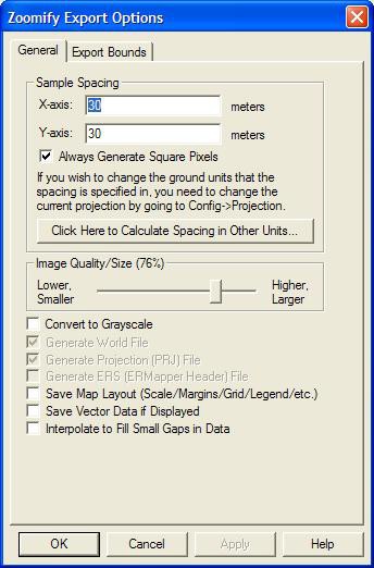
Note:
Only registered users of Global Mapper are able to export data to any format.
Export XY Color Command
The
Export XY Color command allows the user to export any loaded data sets to a
comma-delimited ASCII XY Color file. Each valid sample will be represented as
follows (note for grayscale export there will just be a single grayscale
value):
x-coordinate,y-coordinate,red,blue,green
When
selected, the command displays the XY
Color Export Options dialog which allows the user to setup the export. The
dialog consists of a General options panel which allows the user to set up the
grid spacing and vertical units, a Gridding
panel, and an Export Bounds panel which
allows the user to set up the portion of the loaded data they wish to export.
Note:
Only registered users of Global Mapper are able to export data to any format.
Export XYZ Grid Command
The Export XYZ Grid command allows the user to export any
loaded elevation grid data sets to a
comma-delimited
ASCII XYZ file. Each grid point will be represented as follows (actual
coordinate delimiter is configurable):
x-coordinate,y-coordinate,z-coordinate
When
selected, the command displays the XYZ
Grid Export Options dialog which allows the user to setup the export. The
dialog consists of a General options panel
which allows the user to set up the grid spacing and vertical units, a Gridding panel, and an Export Bounds panel which allows the user to set up the portion of
the loaded data they wish to export.
Note:
Only registered users of Global Mapper are able to export data to any format.
Export Zmap Plus Grid File Command
The Export Zmap Plus Grid File command allows the user to
export any loaded elevation grid data sets to a
Zmap Plus Grid format file.
When
selected, the command displays the Zmap
Plus Grid Export Options dialog which allows the user to setup the export.
The dialog consists of a General options panel
which allows the user to set up the grid spacing and vertical units and an Export Bounds panel which allows the user to
set up the portion of the loaded data they wish to export.
 Note:
Only registered users of Global Mapper are able to export data to any format.
Export Vector Data
Note:
Only registered users of Global Mapper are able to export data to any format.
Export Vector Data
The commands on the Export Vector
Data submenu allow the user to export loaded vector data to various
formats.
Export AnuDEM Contour Command
The Export AnuDEM Contour commands allows the user to export
any loaded contour line data to the
AnuDEM contour .gen file format.
When selected, the command displays the AnuDEM Export Options dialog which consists of an Export
Bounds panel that allows the user to set up the portion of the loaded
vector data they wish to export. Note: Only
registered users of Global Mapper are able to export data to any format.
Export Arc Ungenerate Command
The Export Arc Ungenerate commands allows the user to export
any loaded vector data sets to an Arc
Ungenerate format file.
When selected, the command displays the Arc Ungenerate Export Options dialog which consists of an Export
Bounds panel that allows the user to set up the portion of the loaded
vector data they wish to export. Note: Only
registered users of Global Mapper are able to export data to any format.
Export CDF Command
The Export CDF command allows the user to export any loaded
vector data sets to a CDF (Common Data
Format) file.
When
selected, the command displays the CDF
Export Options dialog (pictured below) which allows the user to set up the
export. The dialog consists of a CDF
Options panel which allows the user to set up the attribute code to assign
to features and the text size in the export file, and an Export Bounds panel which allows the user to set up the portion of
the loaded vector data they wish to export.
If the Use Default
Attribute for All Features option is checked, the attribute selected in the
Default Attribute Code panel will be
used for all features. Otherwise, the selected attribute will only be used for
those features whose Global Mapper classification could not be automatically
mapped to one of the CDF attributes.

Note:
Only registered users of Global Mapper are able to export data to any format.
Export CSV Command
The Export CSV command allows the user to export any loaded
point data sets to a CSV (Comma Separated
File) file.
When
selected, the command displays the CSV
Export Options dialog which allows the user to set up the export. The
dialog consists of an Options panel
which allows the user to set up options such whether or not to include an
elevation attribute for each point as well as whether to include the name of
each column in the file as the first row in the file. There is also an Export Bounds panel which allows the user to
set up the portion of the loaded point data they wish to export.
If
you choose to Export Separate Lat/Lon
Coordinates for Each Point, the LATITUDE and LONGITUDE attributes that are
created will use the current Position Display Format setting on the General tab
of the Configuration dialog for formatting those values if you also have the
option checked to Format lat/lon
coordinates with Position Display Format.
ADVANCED USERS - In
Global Mapper v11.02 and later you can customize the number of decimal digits
written out for the X and Y coordinates for a CSV export by creating a DWORD
registry key
'HKEY_CURRENT_USER\Software\Global
Mapper\ASCIIExportCoordPrecision'. For example, set this value to 6 to get 6
decimal digits for each X, Y, and Z coordinate.
Note:
Only registered users of Global Mapper are able to export data to any format.
Export Delft3D (LDB) Command
The
Export Delft3D (LDB) command allows the user to export any loaded vector line
data sets to a Delft3D (LDB) format file.
When
selected, the command displays the Delft3D
Export Options dialog which consists of an Export
Bounds panel that allows the user to
set up the portion of the loaded vector data they wish to export.
Note:
Only registered users of Global Mapper are able to export data to any format.
Export DeLorme Text File Command
The
Export DeLorme Text File command allows the user to export any loaded vector
features to one of 3 text formats that can be loaded into select DeLorme
mapping products.
When selected, the command displays the DeLorme Text Polygon Export Options dialog which consists of an
Export Bounds panel that allows the user to set up the portion of the loaded
vector data they wish to export. Note: Only
registered users of Global Mapper are able to export data to any format.
Export DGN Command
The
Export DGN command allows the user to export any loaded vector data to a
MicroStation DGN v8 format file.
When
selected, the command displays the DGN
Export Options dialog (pictured below) which allows the user to set up the
export. The dialog consists of a DGN
Options panel, a Gridding panel, and an
Export Bounds panel which allows the user to set up the portion of the loaded
vector data they wish to export.

The
Text Size section allows the user to
control how large display label text will be in the created file. The Unit Resolution value is used to specify
the resolution unit saved in the DGN file. If the Generate PRJ File option is checked, a .prj projection file
describing the projection of the coordinates in the file will automatically be
created. If the Generate 3D DGN File if
3D Features Present option is checked, the entire DGN file will be marked
as 3D and any features that have a elevation data associated with them will be
stored as 3D features. If the Generate
Tags for Feature Attributes option is checked, any attributes associated
with exported features will be saved as tags in the resulting file. Note that
this can significantly slow down your export in some cases. If the Set Global Origin to the Lower Left of
Design Plane Rather than the Center of the Design Plane option is set, the
global origin is set to the minimum valid negative values rather than at (0,0)
as is standard. If the Replace Dark Line
Colors with White option is set, any lines that are near black in color
will be replaced with a white line automatically. This is useful for getting
dark colored lines to show up when the exported DGN file is viewed in an
application that uses a black background.
Note:
Only registered users of Global Mapper are able to export data to any format.
Export DLG-O Command
The
Export DLG-O command allows the user to export any loaded vector data sets to a
native format USGS DLG-O (Digital Line Graph Optional format) file.
When
selected, the command displays the DLG-O
Export Options dialog (pictured below) which allows the user to set up the
export. The dialog consists of a DLG-O
Options panel which allows the user to set up the banner name, DCU (digital
cartographic unit or quad name), and category name, a Gridding panel, and an Export Bounds
panel which allows the user to set up the portion of the loaded vector data
they wish to export. If possible, the fields on the DLG-O Options panel are automatically filled in with the best
guesses available based on the currently loaded data. The user is free to
change the values to fit their needs.

Note:
Only registered users of Global Mapper are able to export data to any format.
Export DXF Command
The
Export DXF command allows the user to export any loaded vector data sets to an
AutoCAD DXF format file.
When
selected, the command displays the DXF
Export Options dialog (pictured below) which allows the user to set up the
export. The dialog consists of a DXF
Options panel, a Gridding panel, and an
Export Bounds panel which allows the user to set up the portion of the loaded
vector data they wish to export.

The
Display Labels section allows you to
control if you want feature display labels included in the DXF files and, if
so, whether you want them represented as TEXT entities in their own layer
(called FEATURE_LABEL) or as DXF attributes. The default is to have them
included as attributes associated with each feature. As some software packages
cannot handle attributes in DXF files, you may have to switch to a different
option (with the associated loss of information) to get your exported DXF files
to work with some software packages. If you would like line features to have
rotated labels running along the line associated with them, you have to use the
option to Include Display Labels as
Separate Text Layer.
The
Layer Names section allows you to
control how the layer names used in the exported DXF file are generated. You
can choose to use the feature description, feature display label, or feature
source filename as the layer name in the exported file. If you choose to use
the display label as the layer name, any features that do not have a display
label will use the feature description as the layer name in the exported file.
If
selected, the Generate Projection (PRJ)
File option causes a projection file describing the ground reference system
of the DXF file to be generated in addition to the DXF file itself. The PRJ
file will have the same
name as the DXF file with the .prj extension.
If
selected, the Create 3D Features Using
Loaded Elevation Data option will cause any underlying elevation data (like
DEMs) to be used to retrieve elevation values for 2D features being exported
and generate new 3D
features in the exported DXF file. The units used by the
elevation values are determined by the Elevation
Display/Export Units setting on the Vertical Options tab of the Configuration dialog.
If selected, the Generate
ECEF Coordinates option will cause the exported DXF file to use
Earth-Centered
Earth-Fixed (ECEF) XYZ coordinate values rather than XY
values in the current export projection.
If
selected, the Generate Zero-Width Lines option
causes and line features created in the DXF file to be marked as having zero
width. Use this option if you intend to use the resulting DXF file with a
product such as MicroStation which has problems with lines of non-zero
thickness.
Note
that if you export features of the TIN
Face Area area type they will be exported as 3D Face features in the
generated DXF file rather than 3D polylines, allowing you to easily get a
usable TIN surface for use in other applications, like 3DS Max.
Note:
Only registered users of Global Mapper are able to export data to any format.
Export DWG Command
The Export DWG command allows the user to export any loaded
vector data sets to an AutoCAD Drawing
(DWG) format file.
When
selected, the command displays the DWG
Export Options dialog (pictured below) which allows the user to set up the
export. The dialog consists of a DWG
Options panel, a Gridding panel, and an
Export Bounds panel which allows the user to set up the portion of the loaded
vector data they wish to export.

The DWG Version section
allows you to select which DWG version to create.
The
Display Labels section allows you to
control if you want feature display labels included in the DWG files and, if
so, whether you want them represented as TEXT entities in their own layer
(called FEATURE_LABEL) or as DWG attributes. The default is to have them
included as attributes associated with each feature. As some software packages
cannot handle attributes in DWG files, you may have to switch to a different
option (with the associated loss of information) to get your exported DWG files
to work with some software packages. If you would like line features to have
rotated labels running along the line associated with them, you have to use the
option to Include Display Labels as
Separate Text Layer.
The
Layer Names section allows you to
control how the layer names used in the exported DWG file are generated. You
can choose to use the feature description, feature display label, or feature
source filename as the layer name in the exported file. If you choose to use
the display label as the layer name, any features that do not have a display
label will use the feature description as the layer name in the exported file.
If
selected, the Generate Projection (PRJ)
File option causes a projection file describing the ground reference system
of the DWG file to be generated in addition to the DWG file itself. The PRJ
file will have the same
name as the DWG file with the .prj extension.
If
selected, the Create 3D Features Using
Loaded Elevation Data option will cause any underlying elevation data (like
DEMs) to be used to retrieve elevation values for 2D features being exported
and generate new 3D features in the exported DWG file. The units used by the
elevation values are determined by the Elevation Display/Export Units setting
on the Vertical Options tab of the
Configuration dialog.
If selected, the Generate
ECEF Coordinates option will cause the exported DWG file to use
Earth-Centered
Earth-Fixed (ECEF) XYZ coordinate values rather than XY
values in the current export projection.
If
selected, the Generate Zero-Width Lines option
causes and line features created in the DWG file to be marked as having zero
width. Use this option if you intend to use the resulting DWG file with a
product such as MicroStation which has problems with lines of non-zero
thickness.
Note:
Only registered users of Global Mapper are able to export data to any format.
Export Esri File or Personal Geodatabase Table Command
The
Export Esri File Geodatabase Table command and Export Esri Personal Geodatabase
Table command allow the user to export any loaded vector data to a table in an Esri File Geodatabase or Esri Personal Geodatabase.
NOTE:
In order to export data to any Esri Geodatabase, you must have installed and
licensed a copy of Esri ArcGIS 9.3.1 or higher. If you do not have ArcGIS
installed, the Esri options will not appear in the selection lists. Support
for Esri Geodatabases is only available in the 32-bit version of Global Mapper.
You can install the 32-bit and 64-bit versions of Global Mapper side-by-side,
and they can share a license.
Note:
Only registered users of Global Mapper are able to export data to any format.
Export Garmin TRK (PCX5) File Command
The
Export Garmin TRK (PCX5) File command allows the user to export any loaded
vector line data to a Garmin TRK (PCX5) format file. This file can be imported
by a wide variety of GPS software, such as Garmin's MapSource®, to
facilitate transferring track logs to a GPS unit.
When
selected, the command displays the Garmin
TRK Format Export Options dialog which allows the user to set up the
export. The dialog consists of an Export Bounds
panel which allows the user to set up the portion of the loaded vector data
they wish to export.
Note:
Only registered users of Global Mapper are able to export data to any format.
Export Garmin WPT (PCX5) File Command
The
Export Garmin WPT (PCX5) File command allows the user to export any loaded
named point data to a Garmin WPT (PCX5) format file. This file can be imported
by a wide variety of GPS software, such as Garmin's MapSource®, to
facilitate transferring waypoints to a GPS unit.
When
selected, the command displays the Garmin
WPT Format Export Options dialog which allows the user to set up the
export. The dialog consists of an Export Bounds
panel which allows the user to set up the portion of the loaded vector data
they wish to export.
Note:
Only registered users of Global Mapper are able to export data to any format.
Export GeoJSON (Javascript Object Notation) Command
The
Export GeoJSON (Javascript Object Notation) command allows the user to export
any loaded vector data sets to a GeoJSON format file.
When
selected, the command displays the GeoJSON
Export Options dialog which allows the user to set up the export. The
dialog consists of an Export Bounds panel
which allows the user to set up the portion of the
loaded vector data they wish to export.
Note:
Only registered users of Global Mapper are able to export data to any format.
Export GOG (Generalized Overlay Graphics) Command
The
Export GOG (Generalized Overlay Graphics) command allows the user to export any
loaded vector data sets to a GOG format file.
When
selected, the command displays the GOG
Export Options dialog which allows the user to set up the export. The
dialog consists of an Export Bounds panel
which allows the user to set up the portion of the loaded vector data they wish
to export.
Note:
Only registered users of Global Mapper are able to export data to any format.
Export GPX (GPS eXchange Format) Command
The
Export GPX (GPS eXchange Format) commands allows the user to export any loaded
point and line data to a GPX (GPS eXchange Format) file.
When
selected, the command displays the GPX Export
Options dialog which consists of an Export
Bounds panel that allows the user to
set up the portion of the loaded vector data they wish to export. If you want
to fill in the <cmt> field of a feature during a GPX export, simply add a
COMMENT attribute to the feature with the desired comment.
Note:
Only registered users of Global Mapper are able to export data to any format.
Export InRoads ASCII Command
The Export InRoads ASCII command allows the user to export
any loaded vector data sets to an InRoads
ASCII format file.
When
selected, the command displays the InRoads
ASCII Export Options dialog which allows the user to set up the export. The
dialog consists of an Export Bounds panel
which allows the user to set up the portion of the loaded vector data they wish
to export.
Note:
Only registered users of Global Mapper are able to export data to any format.
Export Hypack Linefile Command
The Export Hypack Linefile command allows the user to export
any loaded vector line data sets to a Hypack
Linefile format file.
When
selected, the command displays the Hypack
Linefile Export Options dialog which allows the user to set up the export.
The dialog consists of an Export Bounds panel
which allows the user to set up the portion of the loaded vector data they wish
to export.
Note:
Only registered users of Global Mapper are able to export data to any format.
Export KML/KMZ Command
The Export KML/KMZ command allows the user to export any
loaded vector data sets to a KML/KMZ
format file for use with Google Earth.
When
selected, the command displays the KML/KMZ
Export Options dialog (pictured below) which allows the user to set up the
export. The dialog consists of a KML/KMZ
Options panel, a Gridding panel, and an
Export Bounds panel which allows the user
to set up the portion of the loaded vector data they wish to export.

The
3D Line Export, 3D Area Export, and 3D Point
Export sections allow the user to control whether or not area, line, and
point features with elevation values associated with them are drawn at the
terrain surface or at the elevation values associated with the feature. You can
specify whether the elevation values are relative to ground level or sea level
if drawing the features above the terrain. If area features are drawn above the
terrain, the Extrude Areas option
allows you to control whether or not they will also be extruded, which means
they will extend back to the terrain surface, making them look like solid 3D
features. If this option is not checked, the areas will just be drawn in space
as a surface and not a 3D closed object. If the Fake 2D Area Heights to Maintain Area Draw Order option is checked,
exported 2D area features will be assigned fake elevation values in order to
attempt to get them to layer properly when displayed in Google Earth. This is
only
necessary
if you have overlapping areas that do not display in the correct order without
this option checked. If point features are drawn above the terrain, the Extrude Points option allows you to
control whether or not a thin line is drawn from the terrain surface at the
location of the point to the floating symbol above the terrain surface.
Enabling this option makes it easier to locate exactly where a point lies
relative to the surface.
The
Filled Area Translucency section
allows the user to control the degree to which filled polygons are see-through
in the created file.
The
Feature Descriptions section allows you
to setup what is contained in the description for each feature in the generated
file. You can choose to include only the feature description and links to any
files associated with a feature, you can choose to add attributes to this, or
you can choose to provide your own HTML text to use
for the feature description. If you use the HTML text
option, you can embed the values of attributes from the feature in the text by
enclosing the attribute name in percent signs, like %ATTR_NAME%. In addition to
the name of attributes, you can also specify <Feature Name>, <Feature
Desc>, <Feature Type>, <Longitude>, or
<Latitude> as the attribute name to get the feature
display label, description, type name, point longitude, or point latitude
embedded in the result. If you need to embed an actual percent sign in your
result, simply use two percent signs consecutively as an escape sequence.
The following additional options are also available:
• Character Encoding - this option controls the
character encoding value encoded in the header of the
KML file. You will typically just
keep the default of iso-8859-1, but if your loaded data includes text
encoded with a different character set, like UTF-8, you can
select that or even type in your own encoding if something else fits your data
best.
• Create Compressed KMZ File - if this option is checked,
a compressed KMZ file will automatically
be created. This will result in much
smaller files and is highly recommended unless you plan on
manually editing the export result yourself in a text
editor.
• Hide Point Features by Default When Loading File - if this
option is checked, all of the point features
exported to the file will be hidden
by default in Google Earth so as not to clutter up the display with a
bunch of point icons.
• Use Displayed Point Symbols Rather than Push-Pins for
Points - if this option is checked, each point
feature will be rendered with the
same symbol displayed in Global Mapper rather than using the
default push-pin symbol from Google Earth. This will result
in a separate PNG file for each symbol used in the output file being included
with the output data to provide the symbols.
• Display Area and Line Labels - if this option is checked,
each exported line or area feature with a
display label will also be marked
with a clickable placemark displaying the label for that area or line
feature. This is the only way to get line or area features
to display labels in Google Earth.
• Highlight Areas in Google Earth when the Cursor Goes Over
Them - if this option is checked, area
features will highlight when you
move your cursor over them in Google Earth. In addition, if you
checked the option to display area and line labels, the area
label will be hidden until you mouse over the area, at which time the label
will popup.
• Generate Index KML File - if this option is checked,
an additional index KML file will be generated
which indexes all tiles exported by
the export command. This is very useful for dealing with very
large data sets as it will automatically load and unload
individual KML tiles as needed for display in Google Earth, much as a map
catalog does in Global Mapper. With this option you can load massive data sets
into Google Earth and they will still display quickly. The drawing style of the
index tiles is controlled by the selected drawing style for the Coverage/Quad
area type on the Area Styles tab of the Configuration dialog.
For
advanced users, you can also customize what is displayed in the balloon text
that appears in Google Earth when you click on a point. You are able to
customize the <Balloon Style> tag to use text with the string value
stored in the registry (create if it doesn't exist) at
'HKEY_CURRENT_USER\Software\Global
Mapper\KmlExport_BalloonStyle'.
If that value is empty the default setting from Google Earth will be used. Note: Only registered users of Global Mapper
are able to export data to any format.
Export Landmark Graphics Command
The Export Landmark Graphics command allows the user to
export any loaded vector data sets to a Landmark
Graphics format file.
When selected, the command displays the Landmark Graphics Export Options dialog which allows the user to
set up the export. The dialog consists of an Export
Bounds panel which allows the user to set up the portion of the loaded
vector data they wish to export.
Note:
Only registered users of Global Mapper are able to export data to any format.
Export Lidar LAS Command
The
Export Lidar LAS command allows the user to export any loaded 3D vector data
sets (like 3D point clouds loaded from other LAS files) to new Lidar LAS format
files. If the source data came from a Lidar format file, like a LAS or MrSid
Lidar file, the attributes from the original data will be maintained. For other
points, in addition to the base position and elevation, if there is an
INTENSITY attribute available for the point, the value of that attribute will
be exported as the intensity for the point in the exported LAS file. If you
choose the Lidar LAS option then a compressed LASzip (LAZ) file will be
created. This offers lossless compression for Lidar data that makes your Lidar
files much smaller!
When
selected, the command displays the Lidar
LAS Export Options dialog which allows the user to setup the export. The
dialog consists of a Gridding panel, and an
Export Bounds panel which allows the user
to set up the portion of the loaded data they wish to export.
Note:
Only registered users of Global Mapper are able to export data to any format.
Export LMN (Spectra Line Management Node) Command
The
Export LMN (Spectra Line Management Node) command allows the user to export any
loaded line features to a LMN format file for use in applications that support
the LMN format. Attributes named FEATURE_GROUP, FEATURE_TYPE, and FEATURE_REP
are recognized for this export and will be used if present to fill in the
appropriate data fields in the exported file.
When
selected, the command displays the LMN
Export Options dialog which allows the user to set up the export. The
dialog consists of a Gridding panel and an Export Bounds panel which allows the user to
set up the portion of the loaded vector data they wish to export.
Note:
Only registered users of Global Mapper are able to export data to any format.
Export Lowrance LCM Command
The Export Lowrance LCM (MapCreate) command allows the user
to export any loaded vector data sets to a
Lowrance LCM format file for use in Lowrance brand GPS
devices. This allows you to create custom maps
for
Lowrance devices from your data. Type assignment will be done based on the built-in
type assignments. In addition, the MP_TYPE attribute classification used for
Polish MP exports for Garmin devices will also work
for
Lowrance exports, so if you provide custom classifications via the MP_TYPE
attribute the type mapping should work for Lowrance exports as well.
The
LCM export only has support for a limited set of types. Feature types that are
not supported for LCM export will not be added to the generated LCM file, so it
is important to use a built-in type (or a type with a custom MP_TYPE value that
is supported) when exporting to the LCM format. The following is a basic list
of the types of features that are supported:
• Area Types
♦ Lakes
♦ Oceans
♦ Parks
♦ Swamp/Wetland
♦ Urban
Areas
• Line Types
♦ Political Boundaries
♦ Contours
♦ Railroads
♦ Roads
♦ Trails
♦ Streams/Rivers
• Point
Types
♦ Airport
♦ Boat Ramp
♦ Campground
♦ Car Repair
♦ City
♦ Church
♦ Department
Store/Shopping
♦ Gas
Station/Fuel
♦ Hospital
♦ Navaids/Buoys
♦ Pharmacy
♦ Post
Office
♦ Restaurant
♦ School
♦ Water
Features (Spring, Stream, Lake Name)
♦ Wrecks
As
the Lowrance format contains some type settings that cannot be captured with
just a simple Global Mapper type selection or through the assignment of a
MP_TYPE attribute, you can also use a LMC_TYPE attribute to provide a specific
Lowrance type to use for some types. Here is a partial list of the supported
LMC_TYPE attribute values:
• Depth
Contour Line Types
♦ 0x50 -
black, thickness 1
♦ 0x51 -
blue, thickness 1
♦ 0x52 -
dark aqua, thickness 1
♦ 0x53 -
dotted aqua, thickness 1
♦ 0x54 -
white, thickness 1
♦ 0x55 -
black, thickness 2
♦ 0x56 -
blue, thickness 2
♦ 0x57 -
dark aqua, thickness 2
♦ 0x58 -
dotted aqua, thickness 2
♦ 0x59 -
white, thickness 2
♦ 0x5A - black,
thickness 3
♦ 0x5B -
blue, thickness 3
♦ 0x5C -
dark aqua, thickness 3
♦ 0x5D -
dotted aqua, thickness 3
♦ 0x5E -
white, thickness 3
When
selected, the command displays the Lowrance
LCM Export Options dialog which allows the user to set up the export. The
dialog consists of a Gridding panel and an Export Bounds panel which allows the user to
set up the portion of the loaded vector data they wish to export.
Note:
Only registered users of Global Mapper are able to export data to any format.
Export Lowrance USR Command
The Export Lowrance USR command allows the user to export
any loaded vector data sets to a Lowrance
USR format file for use in Lowrance brand GPS devices.
When
selected, the command displays the Lowrance
USR Export Options dialog which allows the user to set up the export. The
dialog consists of a Gridding panel and an Export Bounds panel which allows the user to
set up the portion of the loaded vector data they wish to export.
Note:
Only registered users of Global Mapper are able to export data to any format.
Export MapGen Command
The Export MapGen command allows the user to export any
loaded vector data sets to a MapGen format file.
When
selected, the command displays the MapGen
Export Options dialog which allows the user to set up the export. The
dialog consists of an Export Bounds panel
which allows the user to set up the portion of the loaded vector data they wish
to export.
Note:
Only registered users of Global Mapper are able to export data to any format.
Export MapInfo MIF/MID Command
The Export MapInfo MIF/MID command allows the user to export
any loaded vector data sets to a MapInfo
MIF/MID format file.
When
selected, the command displays the MapInfo
Export Options dialog which allows the user to set up the export. The dialog
consists of a Gridding panel and an Export Bounds panel which allows the user to
set up the portion of the loaded vector data they wish to export.
Note:
Only registered users of Global Mapper are able to export data to any format.
Export MapInfo TAB/MAP Command
The Export MapInfo TAB/MAP command allows the user to export
any loaded vector data sets to a MapInfo
TAB/MAP format file.
When
selected, the command displays the MapInfo
Export Options dialog which allows the user to set up the export. The
dialog consists of a Gridding panel and an Export Bounds panel which allows the user to
set up the portion of the loaded vector data they wish to export.
Note:
Only registered users of Global Mapper are able to export data to any format. Export
MatLab Command
The Export MatLab command allows the user to export any
loaded vector data sets to a MatLab format file.
When
selected, the command displays the MatLab
Export Options dialog which allows the user to set up the export. The
dialog consists of an Export Bounds panel
which allows the user to set up the portion of the loaded vector data they wish
to export.
Note:
Only registered users of Global Mapper are able to export data to any format.
Export Moss Command
The
Export Moss command allows the user to export any loaded area and line vector
features to a Moss format file.
When
selected, the command displays the Moss
Export Options dialog which allows the user to set up the export. The
dialog consists of an Export Bounds panel
which allows the user to set up the portion of the loaded vector data they wish
to export.
Note:
Only registered users of Global Mapper are able to export data to any format.
Export NIMA ASC Command
The Export NIMA ASC command allows the user to export any
loaded vector data sets to a NIMA ASC
format file that can be used on many shipboard radar
displays.
When selected, the command displays the NIMA ASC Export Options dialog which allows the user to set up the
export. The dialog consists of an Export Bounds
panel which allows the user to set up the portion of the loaded vector data
they wish to export.
Note:
Only registered users of Global Mapper are able to export data to any format.
Export Orca XML Command
The Export Orca XML command allows the user to export any loaded
line and point vector data sets to an
Orca XML format file.
When selected, the command displays the Orca XML Export Options dialog which allows the user to set up the
export. The dialog consists of an Export Bounds
panel which allows the user to set up the portion of the loaded vector data
they wish to export.
Note:
Only registered users of Global Mapper are able to export data to any format.
Export OSM (OpenStreetMap.org) XML Command
The
Export OSM (OpenStreetMap.org) XML command allows the user to export any loaded
vector data sets to an OSM XML format file that can be used to provide new data
to the OpenStreetMap.org
web site.
When selected, the command displays the OSM XML Export Options dialog which allows the user to set up the
export. The dialog consists of an Export Bounds
panel which allows the user to set up the portion of the loaded vector data
they wish to export.
Note:
Only registered users of Global Mapper are able to export data to any format.
Export Platte River/WhiteStar/Geographix File Command
The
Export Platte River/Whitestar/Geographix File command allows the user to export
any loaded area features to a Platte River Digitizer/Whitestar/Geographix
Township/Range ASCII format file. These files can be used with several
applications.
When
selected, the command displays the Platte
River Export Options dialog which allows the user to setup the export. The
dialog consists of an Export Bounds panel
which allows the user to set up the portion of the loaded data they wish to
export.
The
township, range, section, and meridian values saved for each area feature
exported are derived either from the attribute values for the area feature or
the display label for "Survey Section" area types. The following
attribute values names are recognized for each field:
• Township
Attributes - TOWNSHIP or TWP
• Township
Direction Attributes - TDIR (must have value of N or S)
• Range
Attributes - RANGE or RNG
• Range
Direction Attributes - RDIR (must have value of E or W)
• Section
Attributes - SECTION, SECT, or SEC
• Meridian
Attributes - MERIDIAN or MER
Note:
Only registered users of Global Mapper are able to export data to any format.
Export PLS-CADD XYZ File Command
The Export PLS-CADD XYZ File command allows the user to
export any loaded vector data sets to a
PLS-CADD XYZ format file. These
files can be used with the PLS-CADD software application.
When
selected, the command displays the PLS-CADD
XYZ Export Options dialog which allows the user to setup the export. The
dialog consists of an Export Bounds panel
which allows the user to set up the portion of the loaded data they wish to
export.
 Note:
Only registered users of Global Mapper are able to export data to any format.
Export Polish MP (cGPSMapper) Command
Note:
Only registered users of Global Mapper are able to export data to any format.
Export Polish MP (cGPSMapper) Command
TUTORIAL ALERT!
Getting Started with Global Mapper
and cGPSMapper - Fantastic Guide to Creating
Garmin-format Maps using Global Mapper, cGPSMapper, and the other supporting
applications required to get your data into a Garmin unit as a new map.
The Export Polish MP command allows the user to export any
loaded vector data sets to Polish MP format files. The Polish MP format is the
input format used by the cGPSMapper application which creates custom maps for Garmin GPS units.
When
selected, the command displays the Polish
MP Export Options dialog (pictured below) which allows the user to set up
the export. The dialog consists of a Map
Options panel, a Gridding panel, and an
Export Bounds
panel which allows the user to set up the portion of the loaded vector data
they wish to export.

The
Map Name and Copyright fields allow to specify the name to use for the final map
when created as well as the copyright text to associate with the map.
The
Map Detail section allows you to
control at what zoom levels the final map will be viewable at. More detail
results in a map that better represents the shape of the source data but that
requires zooming further in to see the map, while less detail will result in a
rougher map that shows up sooner. You should tailer this to the approximate
scale of your source data, will the lowest detail setting approximating source
vector data of around 1:250K scale and the highest detail setting representing
1:24K or better scale data.
Most
built-in types already have a default zoom scale at which they will show up in
built MP maps (this will translate to a Levels= value for the feature in the
exported MP file based on the levels in the MP file header). For custom types
and for types that you want to change the default zoom scale for, you can add a
MP_BIT_LEVEL attribute to the feature itself or to the default attribute list
for a feature type. The value of this attribute should specify the minimum MP
zoom bit level that a feature should appear at. For example, if you use the
maximum Map Detail setting with no
template file, you will get a map with populated zoom levels at 24, 22, and 20
bits. If you wanted a feature to show up in just the lower 2 zoom levels of
that map (the 24 and 22 bit resolution layers), you could add a MP_BIT_LEVEL
attribute with a value of 22 to your feature or the default attribute list for
that type, then that feature would get a Levels=2 value written to the exported
MP file. If your map had less detail (say zoom levels of 21, 19, and 17 bits),
the same feature would
only
show up in the most detailed 21 bit layer as features are always present in at
least one layer of the map. If you want a feature to always show up at all zoom
levels in your map regardless of what zoom levels are present, just add a
MP_BIT_LEVEL attribute with a value of 1.
The
Template File sections allows you to
select a file to use as a template for the new MP file. The new file with use
all of the settings from the selected template file except for the map ID
(unless you check the Keep Image ID from
Template MP File option) and, if you provide a map name, the map name. This
includes the Dictionary setting and all levels settings. This provides a way
for advanced users to set up one MP file exactly how they want and then export
new maps with the same settings. You can also check the Copy Entire
Contents of Template File option to have everything from the template file copied to
the new file verbatim, including any feature data in the template file.
If
selected, the Create as Marine Map option
specifies that the created MP file will be marked as a marine map and marine
features will be used if appropriate. Note that the Marine version of
cGPSMapper is required to create marine maps.
The
Make All Point Features Searchable controls
whether or not all point features in the final map created from the MP file
should be searchable on the GPS device. If the Create Transparent Map option is selected the map will be marked as
transparent and any data under the map will show through.
If
selected, the Save All Attributes (Even
Non-MP Attributes option specifies that all attributes from exported
features will be included in the exported MP file, rather than just those
attributes recognized for that feature type by the MP format. Most users won't
ever need to use this.
When
Global Mapper exports loaded vector data to a MP file, it will automatically
attempt to determine the best type to save in the MP file based on the
classification of the feature in Global Mapper. If no type mapping is known,
the name of the assigned Global Mapper classification will be used for the
'Type' value in the MP file. If you updated your RgnTypes.txt file in your
cGPSMapper folder with the type names and the
appropriate
type number, you can make this work as well. You can also manually specify the
type number to use for a feature by adding an attribute named MP_TYPE with the
type value to use as the attribute value. If the value that you provide is for
a marine type you should also provide an attribute with a name of MARINE and a
value of Y. You can also override the default type mapping for built-in types
by adding a default attribute list for the type on the * Styles tab of the
Configuration dialog. Just add a MP_TYPE attribute to the default attribute
list for a type to manually specify what type to use in exported MP files for a
given Global Mapper type.
Global
Mapper will automatically convert exported data to the appropriate projection
and datum for export so that the Polish MP file will be correctly positioned.
By default this will be lat/lon degrees with the WGS84 datum, although if you
use a template file that specified a different recognized datum, Global Mapper
will instead convert to that datum automatically. In any case, Global Mapper
will always automatically do the right thing.
Advanced
Users: If you aren't use a template to configure your export, you can customize
the values used for several settings in the header for adding registry keys.
The following values are supported:
• TreSize -
Add a DWORD registry value using 'regedit' at
'HKEY_CURRENT_USER\Software\Global
Mapper\MPExport_TreSize' with your desired value.
• RgnLimit -
Add a DWORD registry value using 'regedit' at
'HKEY_CURRENT_USER\Software\Global
Mapper\MPExport_RgnLimit' with your desired value.
Note:
Only registered users of Global Mapper are able to export data to any format.
Export SEGP1 Command
The Export SEGP1 command allows the user to export any
loaded 3D line and point vector data sets to a
SEGP1 format file.
When selected, the command displays the SEGP1 Export Options dialog which allows the user to set up the
export. The dialog consists of a Gridding panel
and an Export Bounds panel which allows the
user to set up the portion of the loaded vector data they wish to export.
Note:
Only registered users of Global Mapper are able to export data to any format.
Export Shapefile Command
The
Export Shapefile command allows the user to export any loaded vector data sets
to ESRI Shapefile format files.
When
selected, the command displays the Shapefile
Export Options dialog (pictured below) which allows the user to set up the
export. The dialog consists of a File
Selection panel, a Gridding panel, and
an Export Bounds
panel which allows the user to set up the portion of the loaded vector data
they wish to export.

The
Export Areas, Export Lines, and Export
Points options enable area, line, and point export respectively. Pressing
the Select... button next to each of
those options allows you to select the name of the SHP file to generate. In
addition to the SHP file containing the actual geometry of the features, an
shape index file (SHX) and attribute database file (DBF) will be created as
well with the same name as the SHP file.
In
general, Global Mapper will automatically determine an appropriate field type
and length for any attributes exported to the DBF file created along with a
Shapefile based on the values of the attribute data being exported. However, if
your input data includes Shapefiles or DBF files, the original field type and
length for an attribute will be used unless the attribute values being exported
make that impossible.
The
Split Export Based On option allows
you to split up your export into separate files based on the feature
type/classification, feature description, feature name, or any attribute found
in the loaded data. If you choose the Split on Feature Type option, you
will get the export split based on the feature classification, except in the
case of the unknown types, in which case the feature description will be used
automatically. The type/description/name/attribute value of the features stored
in each file will be appended on to the end of the selected filenames.
If
selected, the Generate Projection (PRJ)
File option causes a projection file describing the ground reference system
of the shapefile to be generated for each shapefile created. The PRJ files will
have the same name as the SHP file with the .prj extension.
If
selected, the Generate 3D Features Using
Loaded Elevation Data option specifies that 3D objects should be created in
the shapefile. The elevation stored for each vertex/point will be the first of
the following which is available:
• The
elevation associated with the vertex/point in question.
• The
elevation associated with the entire feature being exported. For example, the
elevation of a
contour line.
• The first
elevation obtained by searching the loaded elevation grid layers at the
position of the
vertex/point.
• A value of 0.0 will be used if no
elevation could be obtained via any of the prior methods.
If
selected, the Add Feature Type (LAYER)
Attribute to DBF option specifies that the type description for each
exported feature will be added as a LAYER attribute to the DBF file generated
with the SHP file.
If
selected, the Add Style Attributes to DBF
option specifies that style attributes should be added to the generated DBF
file containing information about the drawing style and label font used for
each feature. If you check this then when you reload your data in Global Mapper
(but typically not other applications) it should maintain its drawing style
If
selected, the Generate Multi-Patch
Features for Areas option specifies that multi-patch features should be
generated for area exports rather than normal polygon records. This is useful
for exporting 3D models, such as those you would load from Google SketchUp SKP
files.
WARNING:
The Shapefile format uses a DBF file for attribute storage, which means that
any attribute names are limited to 10 characters. Any attribute names longer
than that will be truncated with a number potentially added on to maintain
uniqueness among multiple long attribute names.
Note:
Only registered users of Global Mapper are able to export data to any format.
Export Simple ASCII Text File Command
The
Export Simple ASCII Text File command allows the user to export any loaded
vector data sets (i.e. areas, lines, and points) to a delimited ASCII text
file. Each vertex in an area or line and the position of each point will be
represented.
When
selected, the command displays the ASCII
Export Options dialog which allows the user to setup the export. The dialog
consists of an Options panel
(pictured below) and an Export Bounds panel
which allows the user to set up the portion of the loaded data they wish to
export.

The
Options panel allows the user to
specify what character to user to separate the x, y, and z coordinates of each
vertex. In addition, the user can specify that they wish to separate each
vector feature with a blank line or some other custom separator text. The Coordinate Order section allows the user
to control the order in which the X (easting/longitude) and Y
(northing/latitude) coordinates are exported. The export of elevation data is
controlled with the Export Elevations option.
The Include Feature Attributes Before
Coordinate Data and Include Drawing
Style Attributes Before Coordinate Data options respectively control
whether or not feature attributes or feature drawing style information is saved
to the file on the lines preceding the coordinate data
for a feature.
If
elevations are being exported, Global Mapper first looks for an elevation
associated with the vertex being exported. If no elevation is associated with
the vertex, Global Mapper then checks all loaded elevation grid data in reverse
order of display to see if any of them have an elevation at the vertex
location. If so, that elevation is used.
ADVANCED USERS - In
Global Mapper v11.02 and later you can customize the number of decimal digits
written out for the X and Y coordinates for a Simple ASCII Text export by
creating a DWORD registry key
'HKEY_CURRENT_USER\Software\Global
Mapper\ASCIIExportCoordPrecision'. For example, set this value to 6 to get 6
decimal digits for each X, Y, and Z coordinate.
Note:
Only registered users of Global Mapper are able to export data to any format.
Export Vector Spatial Database Command
The Export Vector Spatial Database command allows the user
to export any loaded vector data to a table in a
Spatial Database.
Global Mapper can export vector data to the following
spatial databases:
• Esri
Enterprise Geodatabase (ArcSDE)
• Esri File
Geodatabase
• Esri
Personal Geodatabase
• MySQL
Spatial
• Oracle
Spatial
• PostGIS/PostgreSQL
NOTE:
In order to export data to any Esri Geodatabase, you must have installed and
licensed a copy of Esri ArcGIS 9.3.1 or higher. If you do not have ArcGIS
installed, the Esri options will not appear in the selection lists. Support
for Esri Geodatabases is only available in the 32-bit version of Global Mapper.
You can install the 32-bit and 64-bit versions of Global Mapper side-by-side,
and they can share a license.
Note:
Only registered users of Global Mapper are able to export data to any format.
Export Surfer BLN Command
The Export Surfer BLN command allows the user to export any
loaded vector data sets to a Surfer BLN
format file used by Golden Software's Surfer package to
specify breaklines.
When
selected, the command displays the Surfer
BLN Export Options dialog which allows the user to set up the export. The
dialog consists of an Export Bounds panel
which allows the user to set up the portion of the loaded vector data they wish
to export.
Note:
Only registered users of Global Mapper are able to export data to any format.
Export SVG Command
The Export SVG command allows the user to export any loaded
vector data sets to a SVG (Scalable Vector
Graphic) format file suitable for display on the web.
When
selected, the command displays the SVG
Export Options dialog which allows the user to set up the export. The
dialog consists of an Export Bounds panel
which allows the user to set up the portion of the loaded vector data they wish
to export.
Note:
Only registered users of Global Mapper are able to export data to any format.
Export Tom Tom OV2 Command
The
Export Tom Tom OV2 command allows the user to export any loaded point data sets
to a Tom Tom OV2 format file for use in creating POI databases for Tom Tom GPS
devices.
When selected, the command displays the Tom Tom OV2 Export Options dialog which allows the user to set
up
the export. The dialog consists of an Export
Bounds panel which allows the user to set up the portion of the loaded
vector data they wish to export.
Note:
Only registered users of Global Mapper are able to export data to any format.
Export Tsunami OVR Command
The Export Tsunami OVR command allows the user to export any
loaded vector data sets to a Tsunami OVR
format file for use in the Tsunami software package.
When selected, the command displays the Tsunami OVR Export Options dialog which allows the user to set
up
the export. The dialog consists of an Export
Bounds panel which allows the user to set up the portion of the loaded
vector data they wish to export.
Note:
Only registered users of Global Mapper are able to export data to any format.
Export UKOOA P/190 Command
The
Export UKOOA P/190 command allows the user to export any loaded 3D line and
point vector data sets to an UKOOA P/190 format file.
When
selected, the command displays the UKOOA
Export Options dialog which allows the user to set up the export. The
dialog consists of a Gridding panel and an Export Bounds panel which allows the user to
set up the portion of the loaded vector data they wish to export.
Note:
Only registered users of Global Mapper are able to export data to any format.
Export Vector Spatial Database Command
The Export Vector Spatial Database command allows the user
to export any loaded vector data to a table in a
Spatial Database.
Global Mapper can export vector data to the following
spatial databases:
• Esri
Enterprise Geodatabase (ArcSDE)
• Esri File
Geodatabase
• Esri
Personal Geodatabase
• MySQL
Spatial
• Oracle
Spatial
• PostGIS/PostgreSQL
Export WAsP MAP File Command
The
Export WAsP MAP File command allows the user to export loaded line and area
features to a WAsP MAP format file for use with the WAsP (Wind Analysis and
Application Program) application (http://www.wasp.dk/.
Only
those line features with an elevation and/or valid roughness attributes will be
exported. Only those area features with valid roughness attributes will be
exported. Valid roughness attributes consist of a ROUGH_L and a ROUGH_R
attribute containing numeric values for the left and right roughness for the feature.
If neither
of
those attributes exist but a RV, ROUGHNESS, or ROUGH attribute is available,
that value will be used for both the left and right roughness for that feature.
When selected, the command displays the WAsP MAP Export Options dialog which allows the user to setup the
export. The dialog consists of an Export Bounds
panel which allows the user to set up the portion of the loaded data they
wish to export.
Note:
Only registered users of Global Mapper are able to export data to any format.
Export ZMap+ IsoMap Line Text File Command
The Export ZMap+ IsoMap Line Text File command allows the
user to export loaded line features to a
ZMap+ text format file for use with applications like Landmark Graphics.
and GeoAtlas.
When
selected, the command displays the ZMap+
IsoMap Line Export Options dialog which allows the user to setup the
export. The dialog consists of an Export Bounds
panel which allows the user to set up the portion of the loaded data they
wish to export.
This
format costs of a header for the file, then a header line for each line feature
which has the line elevation (if available), then one line per each input
coordinate, with the X coordinate followed by the Y coordinate. All features
will be tagged as contour line types. The following is short sample of an
output file with a couple of features:
! File exported
from Global Mapper using the ZMap+ IsoMap Line export.
!
! Projection UTM Zone 15 / NAD27 / meters
!
@CONTOUR FILE, CNTR, 80, 1
X (EASTING), 1, 1, 1, 1, 20, 7, 0.1000000E+31, , 20, 7, 0
Y (NORTHING), 2, 2, 1, 21, 40, 7, 0.1000000E+31, , 20, 7, 0
@
0.1000000E+31 245
380262.118 4321646.769
380249.294 4321650.577
380232.064 4321651.300
380222.628 4321653.954
380202.009 4321657.046
380195.088 4321656.460
380171.954 4321657.686
380202.009 4321888.741
380216.955 4321887.882
380232.064 4321887.882
380247.579 4321888.450
380262.118 4321888.450
0.1000000E+31 245
380262.118 4320539.721
380257.495 4320550.684
380254.024 4320555.291
380262.118 4320563.813
Note:
Only registered users of Global Mapper are able to export data to any format.
Export ZMap+ XYSegId File Command
The Export ZMap+ XYSegId File command allows the user to
export loaded line and area features to a
ZMap+ text format file for use with applications like Landmark Graphics..
When
selected, the command displays the ZMap+
XYSegId Export Options dialog which allows the user to setup the export.
The dialog consists of an Export Bounds panel
which allows the user to set up the portion of the loaded data they wish to
export.
This
format costs of one line per each input coordinate, with the X coordinate
followed by the Y coordinate (optionally with a Z if available), followed by
the feature index in the file. The following is short sample of an output file
with a couple of features:
|
924800.1
|
10593255.0
|
1.
|
|
919970.1
|
10590840.0
|
1.
|
|
915623.0
|
10586976.0
|
1.
|
|
914174.0
|
10579248.0
|
1.
|
|
919487.0
|
10573451.0
|
1.
|
|
927215.1
|
10569587.0
|
1.
|
|
933977.3
|
10568138.0
|
1.
|
|
938324.3
|
10575867.0
|
1.
|
|
937358.3
|
10586493.0
|
1.
|
|
934460.2
|
10593255.0
|
1.
|
|
927698.3
|
10594221.0
|
1.
|
|
924800.1
|
10593255.0
|
1.
|
|
884645.6
|
10557271.0
|
2.
|
|
887543.7
|
10549543.0
|
2.
|
|
893822.8
|
10540849.0
|
2.
|
|
900584.8
|
10539400.0
|
2.
|
|
906380.8
|
10543264.0
|
2.
|
|
907829.9
|
10554373.0
|
2.
|
|
900584.8
|
10565965.0
|
2.
|
|
895271.8
|
10567414.0
|
2.
|
|
886094.7
|
10565965.0
|
2.
|
|
884645.6
|
10557271.0
|
2.
|
|
876917.6
|
10524427.0
|
3.
|
|
870155.4
|
10518630.0
|
3.
|
|
865808.5
|
10512834.0
|
3.
|
|
861944.4
|
10503657.0
|
3.
|
|
865325.6
|
10494963.0
|
3.
|
|
871121.6
|
10493997.0
|
3.
|
|
880781.6
|
10496895.0
|
3.
|
|
889475.8
|
10499793.0
|
3.
|
|
890924.8
|
10509936.0
|
3.
|
|
889475.8
|
10518147.0
|
3.
|
|
884645.6
|
10524910.0
|
3.
|
|
876917.6
|
10524427.0
|
3.
|
Note:
Only registered users of Global Mapper are able to export data to any format.
Batch Convert/Reproject
The
Batch Convert/Reproject command allows the user to easily convert multiple
files in one format to another format.
When
the command is selected, the user is first prompted to select the file type to
convert from using the dialog pictured below. Once an input file type is
selected, another dialog with a list of all compatible export file types is
displayed, allowing the user to select what type of file to convert the input
files to. Finally, after
the input and output flle types are selected,
the Batch Convert dialog (pictured below) is displayed, allowing
the user to set up the
batch conversion.
 Select File Type to Convert From

 1Select Type
ACE
(Altitude Corrected Elevation)
Arc Vector Coverage File
Arc/lnfo ASCII
Grid File
Arc/lnfo Binary
Grid File
AutoCAD DXF (Drawing lnterchange File)
BSB

 iJ 1 . _
o_K ,
iJ 1 . _
o_K ,

 " Cancel
 "1 " -----
 Select File Type to Convert
To
Select File Type to Convert
To
Arc/lnfo ASCII
Grid File
---..
Cancel


 !select Type iJ 1 OK
 BIL (Band lnerleaved lmagery)
BIL (16-bit Elevation Samples)
BIL (32-bit Elevation Samples)
BIP (Band lnterleaved Pixel)
BSQ (Band Sequentiallmagery)
 DEM IUSGS ASCII DEM Formatl
Batch Convert
r Source Files rDestinationFiles
rDirectory
G:\DATA\IMAGERY\35NB!JW_Eievation_Drape_1 r. Use same directory as file
1 OK 1
G:\DATA\IMAGERY\Bathurst lnlet North.tif Cancel
G:\DATA\IMAGERY\Burlington Standard NatColor being converted 1
G:\DATA\IMAGERY\Burlington Standard NatColor r Specify output directory. Help
G:\DATA\IMAGERY\C3009213_NWJ_20 2ip Change.
G:\DATA\IMAGERY\NTS95B07_95A03_01_1RS.1
G:\DATA\IMAGERY\compressed_tif_example.tif
G:\DATA\IMAGERY\ev11656_1and_shallow_topo_
1 1
rFile Names
G:\DATA\IMAGERY\isla_chaî'iaral.tif (i" Use
Source File Name
G:\DATA\IMAGERY\s05120a1.tif to Filename
G:\DATA\IMAGERY\seco_resamp_rect.tif
G:\DATA\IMAGERY\smallli2.tif r Use Quad Name
rProjection
r. Use Source File Projection
Specify Projection Change...
1
Setup Gridding (i.e. Tiling)...
1
Setup Sample Spacing...
1
Horz Datum J Source Datum iJ
lli lill' 1 _tl OUse Other Source Files As Filler
Add Files...
Remove Selected
1 1
OGenerate Projection (PRJ) Files
OGenerate World Files (TFW.JGW) =1
Add Directory...
1
Add Loaded Files
RemoveAII
Add OnscreenFiles
1 Force Square Pixels in Output
ORemove Collar From Image
1 1
nAdiust lmaoe Contrast
!YI
The
Source Files section displays the
list of source files currently selected to be converted. Pressing the Add Files... button allows the user to
select additional files for conversion. Pressing the Add Directory... allows the user to easily add an entire
directory's worth of source files to the to-be-converted list. All directories
under
the
added one can be recursively searched if so desired by answering Yes to the
dialog that pops up immediately after selecting the directory. Pressing the Add Loaded Files button causes all files
loaded into the main Global Mapper view that match that batch convert input
type to be added to the list of files to be converted. Pressing the Add Onscreen Files button causes all
files loaded into the main Global Mapper view that are currently at least
partially onscreen and that match the batch convert input type to be added to
the list of files to be converted.
The
Directory section allows the user to
choose where they would like the newly created output files to be created. The Use same directory as file being converted option
causes the output file created off of each
source
file to be created in the same directory as the source file. The Specify output directory option allows
the user to choose a specific directory to output all of the newly created
output files to.
The
File Names section allows the user to
choose whether the newly created output files should have the same file name as
the source file they were created from (Use
Source File Name option) or whether the more readable quadrangle name (if
available) or layer descripiton should be used as the file name for the newly
created output file (Use Quad Name or
Description option). If the Use
Source File Name option is selected, you can also specify an additional
text string to append to each new filename to identify it.
The
Projection section allows the user to
choose whether or not each newly created output file should either use the same
projection as the file that it was created from (Use Source File Projection option) or if each file should use a
projection specified by pressing the Projection
button. If the user selects to specify an output projection and they select
a zoned projection like UTM or Gauss Krueger, they will have the option on the
projection selection dialog to have the best zone for the center of the output
map automatically used if they select the Automatically
Select Best Zone option in the Zone box on the projection selection dialog.
The
Setup Gridding (i.e. Tiling) button
displays a dialog allowing the user to specify if and how to break up each file
being converted into multiple new files. This option is only available when
converting to a raster or gridded elevation format.
The
Setup Sample Spacing button displays
a dialog allowing the user to choose to either keep the sample spacing of
source raster and elevation files when converting the selected or to specify a
new sample spacing to resample all of the selected input files at when
performing the conversion. This option is only available when converting to a
raster or gridded elevation format.
The
Horz Datum selection allows the user
to choose the horizontal datum that each newly created output file should use.
By default, each output file will use the same horizontal datum as the source
file that it was created off of. Alternately, the user can specify to have all
output files created in NAD27, NAD83, WGS72, or WGS84 with the appropriate
offset being applied automatically.
The Vertical Units selection
is present only for some conversions and controls the output elevation units.
The
Palette selection is present only for
some conversions and controls the palette, if any, used in the output files.
The palette values are defined as follows:
• Image Optimized Palette - The palette generated will
be an optimal mix of up to 256 colors that will
closely represent the full blend of
colors in the source images. This option will generate the best
results, but can more than double the export time required
if any high color images are present in the export set. If all of the input
data is palette-based and the combined palette of those files has 256
colors or less, then the combined files of the input file
will just be used with no additional export time being required.
• Grayscale Palette - This palette consists of
256 scales of gray ranging from black to white.
• DRG Optimized Palette - This palette is optimized
for the exporting USGS DRG data. The palette
consists of only the standard DRG
colors.
• DRG/DOQ Optimized Palette - As the name suggests, this
palette is optimized for exporting a mixture
of USGS DRG data and grayscale
satellite photos (i.e. USGS DOQs). The palette consists of the 14
standard DRG colors with the remaining 242 colors being a
range of gray values ranging from black to white.
• Halftone Palette - The palette consists of a
blend of 256 colors evenly covering the color spectrum.
This palette is the best choice when
exporting anything but DRGs and grayscale satellite photos.
• Custom Palette from File - This option allows the
user to choose a .pal file describing the palette to
use for the export. A .pal file
should be a text file with one line per color, with the red, green, and blue
color components for each color in the palette separated by
a comma. You can save a .pal file for an existing palette-based file by opening
the Overlay Control Center, selecting the palette-based layer, press Options,
then the Transparent Color button, then selecting the option to save a color
palette file.
• 24-bit RGB - Create a full 24-bit color image
with no palette. This will create the best resulting image
but will also take the most space.
• Keep Same as Source File - The new file will use the
same color encoding as the source file, either
palette-based, 24-bit RGB,
multi-band, or grayscale.
• Multi-Band Image - The new file will use be a
multi-band image using the same number of bands as
the input file. You will be able to
choose either 8-bits or 16-bits per band.
The
additional list of options varies depending on the particular conversion being
performed. The meaning of those options is defined below:
• Add Watermark Image - when this option is
checked, you will be prompted to select an image to use
as a watermark for your raster
format export. You will also be allows to select display options for
your watermark image, such as transparency, to provide the
desired effect. The selected watermark image will be stretched to cover the
entire output image for each converted file.
• Adjust Image Contrast - causes the contrast of any
input file to be automatically adjusted prior to
being exported. This is useful for
improving the display of some types of imagery.
• Clamp Export to Lat/Lon Boundary - causes
the export bounds of each image being converted to be
clamped to the nearest 3.75' lat/lon
boundary. This can be useful in limited cases, such as when
reprojecting to geographic/arc degrees and the source images
had a tiny collar to make the image square in the native projection.
• Convert to Grayscale - causes the exported
imagery to be generated in only shades of gray.
• Crop to Selected Areas - this option specifies that
each exported file will be cropped to any area
features selected with the Feature
Info or Digitizer Tools. If this option is selected, no output file will
be generated for any input file that does not intersect any
of the selected crop areas.
• Export Areas, Export
Lines, and Export Points - these
options respectively control whether area, line,
and/or point shapefiles are
generated from the source vector data files. At least one of these options
must be selected.
• Fill Small Gaps in Data - this option specifies
whether or not small gaps in the elevation or raster file
being exported will be filled by
interpolating between nearby known values.
• Force Square Pixels in Output - causes
the newly created files to have square pixels in whatever
projection they are created in. This
allows the files to be used with the widest variety of other
software packages, many of which do not correctly handle
non-square pixels.
• Generate Projection (PRJ) File - causes a
projection file describing the ground reference system of
the output file to be generated for
each output file in addition to the output file itself. The PRJ file will
have the same name as the output file with the .prj
extension.
• Generate World File - causes a world file
describing the location of the output file to be generated for
each output file. The world file
will have the same name as the output file with the appropriate world
file extension for the output type (i.e. TFW for GeoTIFF,
JGW for JPEG, etc.).
• Include Display Labels as Attributes - causes
DXF attributes containing the name of the vector object
to be associated with DXF POLYLINE
entities. As some software packages cannot handle attributes
in DXF files, you may have to turn this option off (with the
associated loss of information) to get your exported DXF files to work with
some packages.
• Include Feature Attributes in DBF - causes
the attributes other than layer and elevation of each
feature (if any) to be stored in the
DBF file associated with the generated Shapefile. In addition,
selecting this option will cause the DLG-3 attribute codes
matching each feature to be stored in the
DBF file.
• Include Feature Names in DBF - causes the name of each
feature (if any) to be stored as a NAME
attribute in the DBF file associated
with the generated Shapefile.
• Make Single Color Transparent - allows
the user to select a single color to treat as transparent in the
source data files.
• Minimize Window During Conversion - this
option causes the main map window to immediately be
minimized when the batch conversion
operation begins and stay that way until the operation
completes.
• Never Anti-Alias Pixels (Interpolate) - this
option disables anti-aliasing (interpolation) even for those
layers to which it would normally be
applied by default (like gridded elevation layers) or imagery
being reprojected or resampled.
• Never Automatically Adjust Contrast - this
option disables automatic contrast adjustment even for
those layers to which it would
normally be applied by default (like 16-bit per color channel images).
• Only Generate Metadata Files - causes only metadata files
like world files, PRJ files, and TAB files
to be generated. This is a very
handy way to create metadata files for a large collection of files like
GeoTIFF files in order to use the data in software that
doesn't recognize embedded positioning information.
• Remove Collar From Image - causes the collar of
DRG-style images to be automatically removed
from each image that is converted if
collar bounds can be automatically determined. Note that some
collar may remain in order to make the end result
rectangular if the destination projection in not geographic lat/lon. If you
check this option and the file being converted is also loaded in the main map
view and has some custom collar cropping applied, those collar cropping options
will be used rather than the automatic DRG-style collar setting.
• Skip Existing Output Files - this option causes any
conversion operations for which the default output
filename already exists to be
skipped. This is useful when resuming batch conversion operations that
failed or were cancelled.
• Use Big Endian For Elevations - causes
stored elevations to use the big-endian (Motorola) byte order
rather than the default little-endian
(Intel) byte order.
• Use Lossless Compression - this option causes the
lossless compression method to be used when
generating Global Mapper Grid files.
If it is not checked, some minor loss of data in areas of high
terrain relief will be allowed in order to achieve a higher
compression ratio.
• Use Other Source Files As Filler - causes
all selected source files to be loaded and made available
during export to fill holes in the
main file being converted. This is useful when you have a collection
of files that are being reprojected and you do not want to
have a sliver around the edge of each new file filled with the background color
when the source data does not make a perfect rectangle. You can even mark some
files to only be used as filler by right clicking on them in the Files list and
selecting the appropriate option in the popup menu.
• Use Tile Layout (ADVANCED USERS ONLY) -
specifies that any exported GeoTIFF or JPEG2000
files should be organized in tiles.
For GeoTIFF if this isn't checked the default strip organization will
be used.
You
can also right click on the list of files to convert and choose to save that
list of files to a text file. This can be a convenient way to start a Global
Mapper script to do other processing on the files. Other right-click options
include the ability to remove all archive files, like .zip and .tar.gz from the
list and to fill the source files list with files listed in a text file.
Note:
Only registered users of Global Mapper are able to perform batch conversions.
Print Command
The Print command allows the user to
print the contents of the current view window. When selected the Print
dialog (picture below) is displayed, which allows the user
to set up the print process.

The
Header field allows the user to
specify text to be displayed above the printed map image. This text will be
printed centered above the map image on the printout.
The Footer field
allows the user to specify text to be displayed below the printed map image.
This text will be printed centered below the map image on the printout. The
footer text will default to the text displayed on the status bar for the active
tool, such as the measurement information for the current measurement in the
Measure Tool.
Selecting
the Print in Black and White option
causes the printout to be generated in black and white, rather than full color
even when printing to a color printer. The generated image will be a 256-level
grayscale image.
Selecting
the Use White Background Color option
causes any background areas being printed to be filled with white so as not to
use any printer ink. Uncheck this option is you want the currently configured
background color to be maintained on the printout.
The
Extra Margin Around Printout setting
allows you to specify an extra margin to draw around the output. This is useful
when printing to things like a PDF file that do not have any natural margins
like a printer does.
The Print To Scale option
allows you to specify that you want the printed result to match a certain
scale, like
1:1000.
This means that one inch on the printed paper will correspond to 1000 inches in
the real world. If you choose to print to a certain scale, the printout will be
centered on the center of your current screen view, but the appropriate amount
of information will be rendered to achieve the requested scale.
The
Print To File section allows you to
specify that the printout be directed to an image file rather than to the
printer. This can be handy if you either want to save the results of the
printout to email to someone or post on
a
web site, or you are having trouble printing and would like to print out the
data generated by Global Mapper using another application.
The
Print Bounds panel allows the user to
select exactly what area to print (the default is the current screen contents).
This panel behaves just like the Export Bounds
panel found on most export dialogs.
Print Preview Command
The
Print Preview command allows the user to preview what a printout of the
contents of the current view window would look like.
Print Setup Command
The
Print Setup command allows the user to setup their printer for printing the
current view window. Exit Command
The
Exit command closes the Global Mapper application. View Menu
The View menu offers the following commands:
• Toolbars - Shows or hides the toolbar(s)
♦ Favorites Toolbar
• Status Bar - Shows or hides the status bar
• Background - Allows user to change the background color
• Center on Location - Allows user to recenter the view on a
location
• Properties - Displays Dialog with Properties of Current
Map View
• Full View - Zooms such that all loaded data is visible
• Zoom In - Zooms in on loaded data by a factor of 2
• Zoom In Micro - Zooms in on loaded data by a small amount
• Zoom Out - Zooms out on loaded data by a factor of 2
• Zoom Out Micro - Zooms out on loaded data by a small amount
• Zoom To Scale - Zooms the current view to a given scale
• Zoom To Spacing (Pixel Size) - Zooms the current view to a given pixel size
• Zoom To Selected Features - Zooms to features selected with Digitizer
Tool
• Zoom To View in Google Earth - Open Google Earth to same view
• Save Current View - Saves the current view for later restoration
• Restore Last Saved View - Restores the last saved view
• Restore Last Drawn View - Restores the last drawn view
• Name and Save Current View - Names and saves the current view
• Restore Named View - Restores a previously saved named view
Toolbars
Use
this command to display and hide the Toolbars, which includes buttons for some
of the most common commands in Global Mapper. A check mark appears next to the
menu item when the Toolbar is displayed

Favorites Toolbar
The
Favorites Toolbar (pictured below) provides very convenient one-click access to
many of the commands in Global Mapper, including nearly every Digitizer Tool command and many of the
commands under the other menu commands. The toolbar consists of a drop-down
with the configured Favorite options and commands to setup the Favorites and a
green arrow that you press to active the currently selected command. You can
also use the Ctrl+Enter shortcut key to run whatever the selected command is,
thus creating a single configurable shortcut key. You can also use the Setup Favorites Shortcut Keys option to
bring up a dialog allowing you to assign shortcut keys to any available
command, providing quick keyboard access to nearly any functionality in the
software! The Setup Favorites List option
allows you to select commands to always have available in the Favorites
drop-down list (above the first separator dashed line). The Favorites toolbar
will also remember what you commonly use in the Digitizer Tool and
automatically populate the list with up to 5 commonly used tasks (these are
placed below the specifically selected commands).

Status Bar

The
status bar is displayed at the bottom of the Global Mapper window. To display
or hide the status bar, use the Status Bar command in the View menu.
The left area of the status bar describes actions of menu
items and toolbar icons. The left area of the status bar will also show color
or elevation of the current pixel if it's over a raster image, or the
description of the closest vector overlay component. If the nearest line
feature to the cursor contains recognized addressing information, the address
nearest the cursor will be displayed.
The
right areas of the status bar indicate the current view scale and the current
mouse position in both the global ground reference system and in the Position
Display Format currently selected from the Configuration dialog.
Background
The Background command brings up a color dialog box from
which the user can select a color to be the new background color of your Global
Mapper window. The background color selected will also be used to fill in areas
of no data in exported raster imagery (i.e. GeoTIFF and JPG files).
Center on Location
The
Center on Location command allows the user to manually enter a location to recenter
the view on, providing a quick and easy way to center yourself on a particular
location.
Properties Properties
The
Properties command displays a dialog listing properties about the current view
window. Full View
The
Full View command zooms such that all of the currently loaded overlays fit in
the view window. This command also places the overlays in the center of the
view window.
Zoom In
The
Zoom In command zooms the current view in by a factor of 2. Zoom In Micro
The
Zoom In Micro command zooms the current view in by a small amount. Zoom Out
The
Zoom Out command zooms the current view out by a factor of 2. Zoom Out Micro
The
Zoom Out Micro command zooms the current view out by a small amount. Zoom To
Scale
The
Zoom To Scale command zoom the current view to a user-specified scale. For
example, to make one inch on the screen be equivalent to 1 mile of ground
truth, you would enter a scale of 63360 (this is the number of inches in a
mile).
Zoom To Spacing (Pixel Size)
The
Zoom To Spacing command zoom the current view so that each pixel on the screen
represents a user-specified number of ground units.
Zoom To Selected Feature(s)
The
Zoom To Selected Feature(s) command zooms the current view to the bounds of the
feature(s) that are currently selected with the Digitizer Tool.
Zoom To View in Google Earth
The
Zoom To View in Google Earth command will open a session of Google Earth on
your machine and pan and zoom it to approximately match your current view. Note
that this does require that you have a copy of Google Earth installed.
Save Current View
The
Save Current View command saves the current map view bounds. The saved view can
later be restored by using the Restore Last Saved View command. This feature
allows you to save a view at one spot, then pan and zoom around and load
additional data, then restore your view to the saved spot in one simple
operation.
Restore Last Saved View
The Restore Last Saved View command restore the map view to
the location last saved using the Save Current
View command.
Restore Last Drawn View
The
Restore Last Drawn View command restore the map view to the view that was last
drawn on the main map. You can use this to back up threw recently drawn view
locations and zoom levels.
Name and Save Current View
The
Name and Save Current View command associates the current map view bounds with
a user-specified name. The saved view can later be restored from a list of
named views using the Restore Named View command. This feature allows you to
save multiple views with descriptive names, then easily restore those views at
a later time.
Restore Named View
The
Restore Named View command allows you to restore a previously saved map view.
You can save map views for later restoration using the Name and Save Current
View command.
Search Menu
The Search menu currently provides the following commands:
• Search By Name
• Search By Attributes, Name, and Description
• Search and Replace
• Find Address
• Find Features with Duplicate Attribute Values
Search By Name
The
Search By Name command allows for searching for features in all loaded vector
data by name. When selected, the Find By
Name dialog is displayed.
The
Find By Name dialog displays a list
of all of the vector features (areas,lines, and/or points) whose label starts
with the search string specified in the Search
String field. This field can contain the ? and * wildcard
characters.
In addition, one can control which vector object types (area,line, and/or
point) to include in the search. Double-clicking on an item in the list will
recenter the view on that object and show a bullseye on it (hold down the ALT
key when double-clicking to not show the bullseye).
The
Edit Selected button displays a
dialog allowing the user to modify the name, feature type, and drawing style of
any features selected.
The Delete Selected button
will mark all selected features as deleted.
This
dialog is particulary handy with the GNIS (Geographic Names) database which is
freely available for download.
Search By Attributes, Name, and Description
The
Search By Attributes, Name, and Description command allows for searching for
features in all loaded vector data by attribute value, name, feature index
within the layer, and description/type. When selected, the Search Vector Data dialog is displayed.

The
Search Vector Data dialog displays a
list of all of the vector features (areas, lines, and/or points) which match
the specified Search Criteria. The Search Criteria can be applied to any
attribute value of the loaded features, the display label field, or the
description/type field. Comparisons to the Compare Value can be done either
textually or numerically. For text equal and not-equal searches, the Compare
Value field can contain the
? and * wildcard characters.
In
addition, one can control which vector object types (area, line, and/or point)
to include in the search and also whether to limit the search to those features
that are on-screen.
Once
you have your Search Criteria set how you want for the search, press the New Search button to actually perform
the search and display the matching results in the results list. The results
will be sorted in ascending order by the names of the features by default, but
you can click on any column header to sort the results by the values in that
column. Clicking the same column header again will reverse the order of the
sort. You can also press the Search in
Existing Results button to apply the new search criteria to the existing
results. Using this you can create complicated searches based on multiple
criteria.
Double-clicking on an item in the list will recenter the
view on that object.
The
Edit Selected button displays a dialog
allowing the user to modify the name, feature type, and drawing style of any
features selected.
The Delete Selected button
will mark all selected features as deleted.
If
you right click on the results list, additonal options will appear, such as the
option to select all of the results in the list. If multiple line features are
selected in the results list, when you right click there will be an option to
combine those line features into new line features if the selected lines
connect at their endpoints. Options for copying the selected features to the
clipboard and selecting the selected search results with the Digitizer Tool for
further editing will also appear if any results are selected.
ADVANCED
USERS: You can change the default search string from '*' to whatever you want
by creating a new registry string value with the desired default search string
at "HKEY_CURRENT_USER\Software\Global Mapper\DefaultVectorSearchStr".
Search and Replace
The Search and Replace command allows for searching for a particular
text string in the attributes and name of loaded features and replacing that
with some other text string. When you select the command, the Search and
Replace dialog (pictured below) is displayed, allowing you to setup the
search-and-replace operation.

When
searching, you can either enter a Search Text value of the string to match on,
or you can enter an asterisk (*) to match any non-empty value. You can also use
the asterisk (*) at the start or end of the search string to look for text that
starts or ends with some particular text.
In the Replace Text box you have more options. You can
specify a simple text string to replace the Search
Text with, or you can use a single wildcard to prepend or
append text.
For
example, to prepend the text 'Sample' in front of your search string, enter a
replace string of 'Sample*'. To append the text to your search string, use
'*Sample'. If you want to replace any string that starts with the sequent 'N '
with 'North ', use a search string of 'N *' and a replace string of 'North *'.
Find Address
The
Find Address command displays the Search
for an Address dialog (pictured below) which allows searching for an
address, city, or postal code anywhere in the world.
If
an address is found that matches the requested location, a results dialog (see
sample below) is displayed with the matching location information, as well as
button to allow creating a new point feature at the address location,
re-centering the map view on the address, and copying the address information
to the Windows clipboard for easy pasting into another application.

The
dialog also includes a Geocode Addresses
from File button that allows you to geocode a bunch of addresses at once.
The text file that you select to convert can either contain a list of files
with addresses in the single line form accepted when searching on a single
address, or it can be a comma or tab-delimited file with
named
columns, like Address, City, State, Country, and Zip or Postcode (see the
example file contents below). Note that you are limited to about 5,000 address
searches within a single 24 hour period.
Sequence,Name,Address,City,State,ZIP,Phone
1,McPeak Betty,,North Pole,AK,99705,907-488-4879
2,McPeak P,,Anchorage,AK,99501,907-770-2957
3,McPeak Roger,,North Pole,AK,99705,907-488-8823
4,McPeak Allan,1011 McCay Ave,Mobile,AL,36609,251-633-0931
5,McPeak Bill,395 Dupree Dr,Huntsville,AL,35806,256-837-2657
6,McPeak Carol,5923 Lumsden
Battery Cir,Mobile,AL,36619,251-661-0989
7,McPeak Dwight,5548 Heath Row Dr,Birmingham,AL,35242,205-991-8862
8,McPeak Faye,146 Larkin St,New Market,AL,35761,256-379-5416
9,McPeak Faye,395 Dupree Dr,Huntsville,AL,35806,256-837-2657
When
batch geo-coding, you can choose to either geocode US addresses against an
online database, or to geocode to loaded road data instead. If you choose to
geocode against loaded road data, you must already have road data loaded with a
known address format, like Tiger/Line data in the US, or data with supported
attribute names for addressing information, like R_FROM_ADR, L_TO_ADR,
R_FROM_CITY, L_TO_CITY, etc., so that the data can be geocoded.
Once
you complete a batch geocode operation, the results are displayed in a list in
a dialog (see sample below). The Batch Geocode Results dialog contains buttons
allowing you to create new point features from the matched address results or
to export the results to a new file.

Find Features with Duplicate Attribute Values
The
Find Features with Duplicate Attribute Values command allows you to search
loaded vector features to find those that have duplicate values for a selected
attribute value. You can then view the results and manually edit them, or
choose to automatically assign unique numeric values for the selected attribute
so that duplicates no longer exist.
When
you select the menu item you are first prompted to select which attribute
(including feature name) to search for duplicates on, then the search proceeds
and any duplicate values are display in the Duplicate
Search Results dialog (picture below). This dialog allow you to view the
features with duplicate results and to edit those features or automatically
assign new unique values. You can also press the Delete Duplicates button to
mark
the duplicate features as deleted. When doing this you will have the option to
mark all duplicates (except for the first one) as deleted, or to just delete
the duplicate features that also have duplicate coordinates (this is what
you'll most often want to do).

Help Menu
The Help menu offers the following commands:
• Online Help Command
• FAQ Command
• User's Group Command
• Register Global Mapper Command
• Check for Updates Command
• About Global Mapper Command
Online Help Command
The
Online Help... command open the table of contents for the Global Mapper User's
Manual in your browser window. You must be connected to the Internet in order
to access the online manual.
FAQ Command
The
FAQ... command opens the Frequently Asked Questions (FAQ) for Global Mapper in your
browser window. You must be connected to the Internet in order to access the
FAQ.
User's Group Command
The
User's Group command open the Global Mapper Yahoo User's Group in your browser
window. You must be connected to the Internet in order to access the user's
group.
Register Global Mapper Command
The
Register Global Mapper... command displays the Registration dialog which allows the user to enter their
registration name and code they obtained after purchasing a license for Global Mapper.
Check for Updates Command
The
Check for Updates... command checks to see if a newer version of Global Mapper
than the current version is being used. If so, a dialog describing the new
version is displayed.
Automatically Check for Updates at Startup Command
The
Automatically Check for Updates at Startup... command controls whether or not
Global Mapper ever automatically checks for a new version automatically when
you start it.
About Global Mapper Command
The
About Global Mapper... command displays the About
Global Mapper dialog which contains version and contact information for
Global Mapper.
Export Bounds Panel

The
Export Bounds panel provides several
different method for specifying the subset of the currently loaded data that
the user wishes to export. Each of these methods is described below. Note that
regardless of the method used to specify the bounds, the exported data will be
generated in the currently selection global projection.
All Loaded Data
All
currently loaded data that is compatible with the current export type will be
exported. This is the default selection.
All Data Visible On Screen
All
data that is currently visible in the Global Mapper view window will be
exported. Lat/Lon (Degrees)
Allows
the user to specify the subset to export as a bounding box in
latitude/longitude coordinates. The default values automatically filled in are
the lat/lon bounds of all currently loaded compatible data.
Global Projection
Allows
the user to specify the subset to export as a bounding box using coordinates in
the currently selected global projection system. The default values
automatically filled in are the bounds of all loaded compatible
data.
Corner w/ Size - Global Projection
Allows
the user to specify the subset to export by entering the northwest corner of
the bounding box to export followed by the width and height of the desired area
to export. The coordinates entered must be in the currently selected global
projection system. The default values automatically filled in result in a
bounding box containing all loaded compatible data.
MGRS (Military Grid Reference System) Bounds
Allows
the user to specify the subset to export by entering the northwest and
southeast corners of the bounding box to export in MGRS coordinates. The
default values automatically filled in result in a bounding box containing all
loaded compatible data.
Crop to Selected Area Feature
If enabled, allows the user to crop the export to the
currently selected area feature(s). To use this for supported exports, select
the area(s) that you wish to crop the export to using either the Feature Info
Tool or the Digitizer Tool.
Draw Box 
Pressing
the Draw Box... button brings up the Drag a Box to Select Export Bounds dialog.
In this dialog, simply hold down the left mouse button and drag a rectangle
around the area of the image that you wish to export. If you make a mistake,
just drag another rectangle.
When
you press the OK button, the bounds
of the rectangle that you drew will automatically be inserted into the
appropriate controls in the Export Bounds
panel.
Gridding Panel

The
Gridding panel provides the user with
the means to easily split up data on export into a regularly spaced grid if
desired, using one of the following options:
• No Grid -
This option means that no gridding will be done, only a single file with be
exported with
the full specified export bounds.
This is the default option.
• Specify
Number of Rows and Columns - Specifies that the data should be broken up into
the given
number of rows and columns of tiles.
Every tile will have the same width and height unless you check
the Crop Right and
Bottom Cells to Export Bounds option, in which case the exported tiles
along the right and bottom may be slightly smaller than the other so that no
data from outside the specified export bounds is used.
• Specify
Individual Grid Cell Width and Height - Allows the user to specify the desired
width and
height in ground units that they
wish each grid cell tile to be. Every tile will have that width and
height, which means that the right-most column and
bottom-most row of tiles could go beyond the specified export bounds. If you
specify negative cell width and/or height values, the grid cells will be
snapped to the right and/or bottom edge(s) of the export bounds rather than the
top left.
• Specify
Individual Grid Cell Pixel Size - Allows the user to specify the desired width
and height in
pixels that they wish each grid cell
tile to be. Every tile will have that width and height in pixels,
which means that the right-most column and bottom-most row
of tiles could go beyond the specified export bounds. This option is not
available for vector-based exports since it does not make sense for
those export types.
• Use
Selected Area Feature(s) for Grid Cells - This option will export a file for
each area feature
selected with the Feature Info or
Digitizer Tools. When you select this feature, you will be prompted
to select how to name the files based on each area. You can
choose from using the display label of the area, the filename of the file that
the area was loaded from, an attribute value of the area, or just a simple
sequential numbering scheme. You will also be prompted to choose whether each
export should actually be cropped to the polygonal boundary of the area or
should just use the rectangular bounds of the area's boundary. Note that when
you select a filename to save to after this, the filename portion of the
selected name will be pre-pended to whatever is used as the grid cell name. So
if you want just your selected item (i.e. attribute, name, etc.) and nothing
prepended, only specify a period and then the extension when selecting the base
output filename, like '.jpg' for JPG output.
If
the user chooses to breakup the data into a grid, then the options in the Grid Naming section will apply and allow
the user to control how the individual grid tile files are named. The following
naming options are available:
• Sequential
Numbering (Row-Major Order) - With this option, a number starting at 1 for the
top-left
tile will be appended to the
selected export filename. The number will increase across each row.
• Separate
Row/Column Letters or Numbers - With this option, separate indicators will be
appended to
the selected export filename for the
row and column. If letters are selected, the letters A-Z will be
used. If more than 27 letters are needed, multiple letters
will be used (e.g. AA, AB, etc.). If numbers are used, the number values will
be pre-pended with zeroes in order to make the numeric values have the same
number of characters for every output tile. If the Reverse checkbox is marked, the order or the numbers or letters used
will be reversed (e.g. if there are 4 rows and numeric naming is selected, the
rows will be named 4, 3, 2, 1 instead of 1, 2, 3, 4). The user also has the
option of specifying the letter/number to start naming at as well as the option
to specify a prefix for each column and row number for each tile and the option
to specify by what value numeric names should change by (step) for each
successive row or column. If the Reverse
Naming option is checked, the column name will come before the row name in
the export filename, otherwise the row name will be before the column name. If
the Prepend 0 to Numbers to Make Same
Length option is checked, the longest number will be found for both the
column and row names and all other column/row names will have 0's prepended to
make them all the same length. The same applies to column/row names using
letters if the Prepend A to Letters to
Make Same Length option is checked. If the Create Folders for Each Row (or Col if Reversed) option is checked,
a separate output sub-folder will be created for each row (or column)
that is exported, preventing too many files from being
placed in a single folder. The Separate
Rows and Columns with Underscore option causes an underscore to be used to
separate row and column values in the output filenames. If not checked then no
separator character will be used.
The
Grid Cell Overlap section allows the
user to specify that the generated grid cells should overlap each other by a
certain percentage of the cell size. This option is useful for loading the
slightly overlapping result files into something like Photoshop for color
matching between cells.
If
the Skip Existing Files option is
checked, any grid cell file that already exists at the destination location
will be skipped. This makes it easy to resume a cancelled export as the already
exported files would not be
re-exported.
Elevation Export - General Options Panel

The
General panel allows the user to
specify the quadrangle name (DEMs only), vertical units, and grid spacing of an
elevation grid being exported.
The Quadrangle Name field
allows the user to enter the quad name to place in the header of a native
format
USGS DEM being exported.
The
Vertical Units field allows the user
to select the vertical units to use when exporting the data (i.e. meters or
feet). Any input data not in the selected vertical units will be automatically
converted on export.
The
Resolution section allows the user to
selected the grid spacing to use when generating the elevation data set. The
default value is the average of the grid spacings of all the currently loaded
elevation overlays.
When
selected, the Interpolate to Fill Small
Gaps option specifies that small gaps in between and within the data sets
being exported will be filled in by interpolating the surrounding data to come
up with an elevation for the point in question. This is useful when data sets
do not line up exactly and so have small gaps in between them.
Image Rectification (Georeferencing)
The Image Rectification feature in Global Mapper allows you to load and work with any JPG, PNG, or
TIFF
imagery, regardless of whether or not spatial positioning
information is provided with it.
For
example, you could scan in an image of a map to a JPG file, use the
File->Rectify Imagery menu command to enter the coordinates of several
points on that image, and then load it into Global
Mapper, properly overlaid with any other loaded data.
Click Here for a Video Tutorial provided by www.globalmapperforum.com
Once
you have rectified an image in Global Mapper,
you can then export it to any of the supported export formats to obtain a fully
rectified image that can then be immediately loaded into numerous other imaging
and GIS packages.
If
you find that after rectifying a file that you want to modify the rectification,
you can simply select the layer in the Overlay
Control Center, then right-click and select the Modify Layer
Position/Projection option to bring up the rectification dialog for that layer.
As-Needed Rectification
There
are two ways to rectify imagery in Global
Mapper. The first is to simply load the imagery file needing to be
rectified just like any other file. Global
Mapper will automatically prompt you to rectify an image if it cannot
automatically determine where on the earth the image should be placed.
If
you indicate that you would like to rectify an image when prompted, the Image Rectifier dialog will appear, allowing
you to enter ground control points for the image in order to rectify it. This
process is described in detail later.
Batch Rectification
By
using the Rectify (Georeference) Imagery command under the File menu, you can
select multiple images to rectify at a time. You will be allowed to rectify all
images that you select, regardless of whether they already contain valid positioning
information. In this way, you can correct poorly positioned imagery.
Using
the Batch Image Rectification Options dialog (pictured below), you can setup
whether you would like to view the images after rectification, export them to
one of several formats, or both.

Regardless
of which options you select, you will then be allowed to rectify each image in
turn using the Image Rectifier dialog, while is described in detail later. As you rectify each image, it will get added to the Reference
Images view in the Image Rectifier dialog,
allowing you to select ground coordinates from it for subsequent images. This
allows you to ensure a good fit between adjacent data files.
If
you selected to save the image(s) to JPG or GeoTIFF image(s), the new files
will be written after you have rectified ALL of the selected files. This is
extremely useful as you can setup the rectification parameters for numerous
images, then let the sometimes lengthy rectification and saving process happen
while you do something else. All newly rectified files will be created in the
same directory as the original images, with
_rectified
appended just before the file extension. The original imagery will remain
intact and unchanged. Image Rectifier Dialog

The
Image Rectifier dialog is the heart of the image rectification process. This
dialog contains everything that you need to rectify an image, from graphical
views of the image, to lists of ground control points, to an
Options
menu for selecting the rectification and resampling methods to use. Each part
of this dialog is covered in detail below.
File Menu
The
File menu provides options allowing you to save the current ground control
point list to a file and to add additional ground control points from a file.
The file specifying the ground control points should be a
comma-delimited file in the following format:
<x-pixel
location>,<y-pixel location>,<x-ground
location>,<y-ground location>,<point name
(optional)>,<point error in pixels (optional)>
There
are also options on the File menu for loading control points and projection
information from an OziExplorer .map, CompeGPS .imp, and Touratech TTQV .cal
files as well as saving your control point information to world (TFW, JGW,
etc.) files.
Options Menu
The Options menu allows you to setup various options related
to the rectification process, as described below:
• Rectification Method - the Rectification Method
submenu allows you to select which rectification
method (hence the name) to apply to
the entered control points. Different methods are available based
on how many control points have been entered. The various
methods are as follows:
♦ Automatic - the Automatic select automatically
selects the "best" rectification method that is
available based on the number of
control points that have been entered. This is the default
method and should rarely need to be changed.
♦ Linear - the Linear rectification method is
used when only two control points are entered.
This is the simplest of the
rectification methods and is equivalent to supplying a world file for
the image. This method does not allow for any distortion or
rotation in the image, but often works well if the correct projection is
selected for the image.
♦ Helmert - the Helmert, or similarity,
rectification method requires at least two controls points
to be entered. This rectification
method is useful if you need to maintain the original shape of
data after a transformation. This method will only be used
if you explicitly select it from the list of rectification methods.
♦ Affine - the Affine rectification method
requires at least three controls points to be entered.
This rectification method calculates
a best fit to a simple equation of the control points
entered. This method can account for some degree of rotation
and distortion, but not with a high degree of accuracy. Because a best fit
approximation is used, some of your ground points may move a little in order to
minimize the error among all control points.
♦ Polynomial - the Polynomial rectification method
requires at least four control points to be
entered. This rectification method
calculates a best fit to a more complex polynomial equation
described the transformation from pixel space to ground
coordinate space. Because a best fit approximation is used, some of your ground
points may move a little in order to minimize the error among all control
points. If you have 6 or more control points, a second order (N=2) polynomial
will be used to transform the points.
♦ Triangulation - the Triangulation
rectification method requires at least five control points to
be entered. This rectification
method performs a Delaunay triangulation for the control points
and will exactly preserve the location of each entered
control point. Occasionally the Triangulation method generates some odd results
around the edges of the rectified image. If this happens, try to enter more
control points around the edge of the image, or change your rectification
method to Polynomial.
• Resampling Method - the Resampling Method
submenu allows you to select how the source image
pixels will be resampled to create
the rectified imagery. These settings simply control which
resampling method is applied initially for rectified images.
This can be changed later in the Overlay
Control Center.
♦ Nearest Neighbor - simply pick the closest
pixel from the source image for each pixel in the
rectified image. This can result in
some blockiness.
♦ Bilinear Interpolation - performs a weighted
average of the four closest pixels in the source
image to determine the color for a
pixel in the rectified image.
• Auto-Name GCPs - this setting controls
whether or not you will be prompted to enter a name for each
ground control point (GCP) entered.
Disabling this allows you to specify a name for each GCP, but
can interrupt workflow. Unless you have a specific need to
name your GCPs, we would recommend turning this option on.
• Display GCP Labels - this setting controls
whether or not the names of each ground control point
(GCP) will be displayed in the
Zoomed and Reference Image views.
• Remember Last Projection - this setting controls
whether or not to initialize the projection to the last
used rectification projection when
rectifying new data. If this is not enabled, the projection will
always default to Geographic/Arc Degrees/WGS84.
• Add Control Points at Corner Points - this
option allows you to easily create a control point at each
corner of the layer being rectified.
If enough other control points have already been entered to do a
rectification, the new corner control points will
automatically be initialized with the best guess at the ground/projected
location, otherwise they will be initialized with dummy values.
• Display Transformation Equations - this
option displays the actual transformation equations used for
transforming this image based on the
selected rectification method and the entered control points.
Note that this is only available if enough control points
have been entered for a transformation to be calculated and if the
transformation method is based on a simple set of equations.
• Show Crosshairs Across Entire Map - this
option controls whether or not crosshair lines are displayed
across the entire Zoomed View and
Reference Image views.
• Automatically Save GCP File When Done - this
option will automatically prompt the user to save a
GCP file when they select the OK or
Apply button to complete a rectification operation.
• Ctrl+Left Click Recenters and Zooms Other View - this
option controls whether or not Ctrl+Left
Clicking in the Zoomed or Reference
Image view just recenters the other view if possible, or if it also
zooms the other view to the same approximate extents.
Entire Image View
The
Entire Image View portion of the Image Rectifier dialog displays, as you might
expect, a view of the entire image being rectified. Any ground control points
(GCPs) will also be depicted on this view with a "big red X". The
current portion of the image being displayed in the Zoomed View section will be
highlighted as well.
You
can use the mouse in the Entire Image View to control what portion of the image
is visible in the Zoomed View. Clicking the left mouse button anywhere in the
Entire Image View will cause the Zoomed View to be recented on the click
position. Dragging a rectangle with the left mouse button will cause the Zoomed
View to recenter and zoom to the box. If you also hold down the CTRL key when
clicking the left mouse button, the Reference Image view will also be
recentered on the associated point if there have been enough control points
entered to convert the coordinates.
Zoomed View
The
Zoomed View portion of the Image Rectifier dialog allows the user to pan and
zoom around the image as well as select pixel coordinates for control point
entry. Any ground control points (GCPs) will be depicted in this view as well
with a "big red X".
You
can drag a box with the left mouse button to zoom in on a particular area in
this view. Right clicking will zoom out. If you hold down the CTRL key when
right-clicking will zoom out to the full extents. For those of you with
wheel-mice, rolling the wheel forward zooms in and rolling it back zooms out.
Moving the mouse near the edge of the Zoomed View displays a pan arrow.
Clicking when this is visible will cause the view to pan in the direction of
the arrow (hold down CTRL to increase the size of the pan). Pressing down the
Shift button while moving the mouse will disable this functionality and allow
you to click all the way to the edge of
the Zoomed View.
To
select a location for control point entry, position the crosshair over the
pixel of interest, then press and release the left mouse button. This will
cause the pixel coordinates of the point to be entered in the Ground Control
Point (GCP) Entry portion of the dialog (described below). In addition, a small
red dot will be placed at the click location to make it easy to see. If you
also hold down the CTRL key when clicking the left mouse button, the Reference
Image view will be recentered on the associated point and the reference
coordinates wil automatically be filled in if there have been enough control
points entered to convert the coordinates. If you hold down the SHIFT key when
left-clicking, the current control point will automatically be added to the GCP
list, just as if you had pressed the Add GCP to List button.
Reference Images
The
Reference Images portion of the Image Rectifier dialog allows the user to view
what is currently loaded in the main Global
Mapper view and to enter ground coordinates by left-clicking on an
appropriate place on the view. This can be very useful for doing things such as
rectifying a satellite photo by clicking on the Zoomed View at a road intersection
to select the pixel coordinates, then clicking on the intersection of those
roads on a vector file loaded into the main view. By default when you click
near a vector feature in the
Zoomed
View, the location will snap to that vector feature. You can disable this
behavior by holding down the ALT key when clicking. If you hold down the SHIFT
key when clicking, the clicked coordinates will be rounded to the nearest 30
seconds for arc degree units and the nearest 1000 ground units for other
coordinate units. Holding down the CTRL key when clicking the left mouse button
will cause the Zoomed Image view will be recentered on the associated point and
also fill in the pixel X and Y coordinatess automatically if there have been
enough control points entered to convert the coordinates.
You can also zoom and pan the Reference Images view in a
manner identical to the Zoomed Images view.
Ground Control Point (GCP) Entry
This
portion of the dialog is where you actually enter the ground control points
(GCPs) that define where the image is on the earth. Typically, you will click a
position in the zoomed view to fill in the pixel coordinates, then manually
enter the ground coordinates into the X/Easting/Lon
and Y/Northing/Lat data fields or
else select a point from the Reference Image view for the ground coordinates.
IMPORTANT:
If you manually enter the ground coordinates, you must enter them in the
coordinate system indicated by the Ground Control Point Projection portion of
the dialog, otherwise you will get incorrect results. The one exception is that
if you enter a value that looks like a lat/lon coordinates but a projected
system is selected, you will be prompted to select whether or not the entered
coordinates are lat/lon coordinates or coordinates in the selected projection
system.
Once
the coordinates are entered, press the Add GCP to List button to add the GCP to
the list of GCPs to be used when rectifying the image. The Update Selected GCP
button allows you to update the coordinates associated with a previously
entered GCP. You can also use Alt+R to simulate pressing the Update Selected
GCP button.
Ground Control Point (GCP) Projection
This
portion of the dialog allows you to select the projection that ground
coordinates are entered in as well as what projection the image will be
natively treated as when rectified (it can be reprojected later using the
normal Global Mapper reprojection
mechanisms). See the IMPORTANT note above for more details.
When
rectifying new imagery, you can control the default projection used by creating
a default_rectification.prj file in your Global Mapper installation folder. If
present, the default rectification projection selected when you open the
rectification dialog will be whatever projection is specified in that PRJ file.
Ground Control Points List
This
section of the dialog contains a list of all of the entered GCPs, including
their name, pixel coordinates, ground coordinates, and the estimated error (in
pixels) at each GCP based on the current rectification method.
Each
GCP has a checkbox next to indicating whether or not that GCP is used for the
rectification. This provided you an easy way to remove GCPs from a
rectification to see how they affect it.
Double-clicking
an item in this list will cause the Zoomed View to recenter on the GCP and will
fill in the Ground Control Point Entry section with the pixel and ground
coordinates of the selected GCP, allowing for easy updating of GCP locations.
You
can move the selection in the GCP list up and down using the Alt+Q and Alt+Z
hot keys. These can help facilitate quickly entering lots of GCPs without
having to use the mouse.
If
you simply want to shift an image, all that you need to do is press the Shift
All button and specify the adjustment to apply to each entered GCP.
Completing the Rectification Process
Once
you have entered all of your ground control points (GCPs), press the OK button
to complete the image rectification. Depending on how you entered the dialog,
the rectified image will now be in the view, will be saved to a new rectified
file, or you will start the rectification of the next selected image.
If you are repositioning a loaded file, you can press the
Apply button to re-rectify the file with the updated
GCPs and see the results of your modifications.
4 LOADING FILES
Choose
[Open as New] icon from the Toolbar. An open window will appear. This window
can be set to display only files of selected types with the "Files of
Type:" subwindow.

There
is support for opening USGS DLG-O, DEM, and several other file types directly
from gzipped archives. In addition, SDTS DLG, SDTS DEM, and most other file
types can be opened directly from .tar.gz,
.tgz,
and .zip archive files. This means that you no longer need to extract all of
those SDTS files to their own directory before opening them. Global Mapper will
do that automatically.
Loading Multiple Files
Global
Mapper will display multiple data sets in correct geospatial positions; that
is, adjacent data sets can be mosaicked, and vector data can be displayed on
top of raster and elevation data.
Choose
[Open Data Files] icon from the Toolbar and select files. The registered
version Global Mapper has no limit on the number of overlays that can be viewed
simultaneously. A maximum of four files of any type may be viewed
simultaneously in the unregistered version of Global Mapper.
You
can also load all of the files under a directory and all subdirectories under
that directory that match a specified filename mask. You can do this using the
[Open All Files in a Directory Tree] File menu command.
Projections and Datums
The
Global Mapper display space adopts the coordinate system of the first data set
opened. Subsequent data sets will be transformed to the coordinate system of
the first data set loaded or the display projection subsequently selected from
the configuration dialog.
This
is a very powerful feature; it makes differences in projections and datums
transparent to the user. This also means that the order in which data sets are
loaded can have a significant impact on the appearance of the display. This is
the most obvious when working with data sets of widely varying scales.
SPATIAL DATABASE SUPPORT
Global Mapper can import vector data from and export vector
data to the following spatial databases:
• Esri
ArcSDE Geodatabase
• Esri File
Geodatabase
• Esri
Personal Geodatabases
• MySQL
Spatial
• Oracle
Spatial
• PostGIS/PostgreSQL
• Spatialite/SQLite
Global Mapper can import raster data from and export raster
data to the following spatial databases:
• Esri
ArcSDE Geodatabase
• Esri File
Geodatabase
• Esri
Personal Geodatabases
NOTE:
In order to import data from an Esri ArcSDE geodatabase or export data to any
Esri geodatabase, you must have installed and licensed a copy of Esri ArcGIS
9.3.1 or higher. Support for Esri Geodatabases is only available in the
32-bit version of Global Mapper. You can install the 32-bit and 64-bit versions
of Global Mapper side-by-side, and they can share a license.
Loading Data from a Spatial Database
There are two ways to load data from a spatial database:
1. Specify the connection parameters for the spatial
database connection. This applies to all of the enterprise databases: ArcSDE,
MySQL, Oracle, and PostGIS. Use the Connection
Manager to define spatial database connections. You can access this
functionality by choosing Open Spatial Database... from the File menu.
2. Specify the file that contains a Spatialite database
(*.sqlite), an Esri file (gdb) or personal geodatabase (*.mdb), or an Esri
ArcSDE geodatabase connection definition (*.sde). Use Esri ArcCatalog or ArcMap
to create an ArcSDE geodatabase connection file. Choose Open Data File(s) from
the File menu to perform this task.

The
Open Spatial Database dialog allows the user to select the connection
parameters that will be used to open an enterprise spatial database.
The Name drop-down
list contains all of the spatial database connections that are currently defined.
Click
the New... button to define a new spatial database connection. When the
button is clicked, the Database Connection Dialog will be displayed. After you
finish setting up a new connection, that name of that connection will be added
to the list and become the selected connection.
The User field
specifies the user ID required to connect to the database. If the selected
database connection
has
a predefined user ID, then that value will be displayed in this field. You can
override this value, if needed. If you type in a different user ID, the stored
database connection definition will not be changed.
Use
the Password field to specify the
password required to connect to the database. If the selected database
connection has a predefined password, then that value will be automatically
entered into this field. You can override this value, if needed. If you types
in a different password, the stored database connection definition will not be
changed.
After
you have selected a connection and entered a user ID and password, click the Open
button to bring up the Spatial Database
Import Options Dialog to choose a table from the database.
The
Cancel button quits the process of opening a spatial database. The Help
button displays the Global Mapper help
for this dialog. Spatial Database Import Options
The
Spatial Database Import Options dialog is used to choose the table or
tables to be loaded from a spatial database. Global Mapper displays this dialog
after you have chosen a spatial database connection, a Spatialte database, an
Esri file geodatabase, an Esri personal geodatabase, or an Esri ArcSDE
geodatabase connection file.

The table list contains the names of the tables in the spatial
database. Put a check next to one or more table(s)
to indicate which tables you want to
load.
Click the Check All button to
place select all of the tables in the list.
Click the Clear All button to remove the check mark
from all of the tables in the list. Once you have marked the tables to be
loaded, click the OK button to load the tables. The Cancel button
quits the process of opening a spatial database.
The Help button displays the Global Mapper help for this dialog.

If the spatial database being opened contains elevation data
or raster imagery, the Spatial Database Import
Options dialog will contain a tab to specify
raster options.
Under
Elevation Options, choose the Vertical Unit for the elevation data.
The default is meters. If you don't choose the correct unit here, you can
always fix it in the Control Center.

If
the spatial database being opened contains vector data, the Spatial Database
Import Options dialog will contain the Import
Bounds tab. This tab allows the user to select a subset of the input data
based on a bounding box. All geometries that intersect the bounding box will be
imported into Global Mapper. This functionality applies only to vector data
in a spatial database.
You can specify the bounding box in the following ways:
• Choose Load
All Data to load all of the data in the selected database tables into
Global Mapper.
• Choose Use
Current Screen Bounds to use the current Global Mapper screen bounds as the
to define
the input bounds. If there is no
data loaded into the viewer, then this option will not be available. If
there is data loaded in Global Mapper, but the full extent
of the data is on the screen, then this option will no be available.
• Click the Draw
a Box... button to draw the bounding box on the screen using your mouse. If
there is
no data loaded into the viewer, then
this option will not be available.
• Choose Lat/Lon
(Degrees) to specify the northwest and southeast corners of the bounding
box in
degrees of latitude and longitude.
• Choose Global
Projection to specify the northwest and southeast corners of the bounding
box in the
unit of the current global
projection. If there is no data loaded into the viewer, or the viewer currently
has no projection defined, then this option will not be available.
• Choose Corner
w/Size - Global Projection to specify the northwest corner, and the width
and height
of the bounding box in the unit of
the current global projection. If there is no data loaded into the
viewer, or the viewer currently has no projection defined,
then this option will not be available.
• Click the Reset
to Last Import Bounds button to retrieve the most recently defined bounding
box in
the unit of the current global
projection. If there is no data loaded into the viewer, or the viewer
currently has no projection defined, then this option will
not be available.
Projections and Datums
The Global Mapper display space adopts the coordinate system
of the first table opened (assuming that there
is
currently no data loaded.) Subsequent data sets will be transformed to the
coordinate system of the first data set loaded or the display projection
subsequently selected from the configuration
dialog.
Exporting Data to a Spatial Database
In
order to export data to a spatial database, you need to specify the location of
the spatial database and one or more table names in which the data will be
stored. When writing to an Esri file geodatabase or personal geodatabase, you
can create a new database file before writing the tables. If you are exporting
data to any of the enterprise database types, you can only create tables in an
existing database.
To export data to a spatial database, you start by choosing
one of the following export options from the
File/Export menu:
• Export Elevation
Spatial Database...
• Export
Raster Spatial Database...
• Export
Vector Spatial Database...
When the Select Export Format Dialog is displayed,
there will be three choices:
• Esri File
Geodatabase Table
• Esri
Personal Geodatabase Table
• Spatialite
DB Table
• Spatial
Database Table
Choose the option indicating your desired spatial database
type, and press OK to continue.
If
you choose Spatial Database from the
list, Global Mapper will display the Open
Spatial Database Dialog. Select the database connection that you want to
use, and click OK to continue by specifying Spatial Database Export Options.
If
you choose Spatialite DB Table, Esri File Geodatabase Table or Esri Personal Geodatabase Table, Global
Mapper will display the Select Esri Geodatabase
Dialog. The following sections describe that dialog and the required steps
to export a table.
Selecting a Spatialite database, Esri File Geodatabase, or
Personal Geodatabase for Export
Use
the Select Database Dialog to choose a Spatialite database, Esri file
geodatabase or personal geodatabase where you want your exported data to be
stored. You can also create a new database, if necessary.

You
can enter the full path to a Spatialite, file geodatabase or personal
geodatabase in the Database field, or
click the Browse... button to select an existing database from the file
system. If you are selecting a Spatialite
database or a personal geodatabase,
then Global Mapper will display the standard Open File dialog. Spatialite database
files have an extension of .sqlite, and personal geodatabase files have an
extension of
.mdb.
If you are selecting a file geodatabase,
Global Mapper will display a Folder Selection dialog. Folder names that end in
.gdb contain file geodatabases.
If
you want to create a new database, click the Create New Database... button.
Global Mapper will display the Create Database Dialog. Once you have
created a new database, the full path will be in the Database field.
Once you have selected a database, click the OK button
to continue by specifying Spatial Database
Export
Options.
The
Cancel button quits the process of exporting data to a spatial database.
The Help button displays the Global
Mapper help for this dialog.
Creating a Spatialite Database, Esri File Geodatabase or
Personal Geodatabase for Export
Use
the Create Database Dialog to specify the location and name for a new
Spatialite database, Esri file geodatabase or personal geodatabase.

Type the full path of the folder where the new database will
be located in the Location field, or
use the
Browse... button to
choose a folder from the file system.
Type
the database name in the Name field.
You do not need to add a file extension -- one will be created automatically
based on the kind of database being created.
Once
you have entered both the location and database name, click the OK button
to create the database. The Cancel button quits the process of exporting
data to a spatial database.
The Help button displays the Global Mapper help for this dialog.
Spatial Database Export Options
Use
the Spatial Database Export Options Dialog to specify the table name(s)
and data extents to be used for this data export. A spatial database table is
restricted to a single geometry type. This dialog allows you to specify table
names for polygon, line, and point geometries based on the data types that are
currently in the display.

On
the Table Selection tab for vector
data export, you can specify a table name for each of the data types that are
currently in the viewer. Note that if you choose an existing table, the data in
that table will be replaced with the data in the viewer.
1. To export polygon features, check the Export Areas box, and enter a table name
in associated entry field. If you want to export data to an existing table,
choose the name from the drop-down list.
2. To export line features, check the Export Lines box, and enter a table name in associated entry field.
If you want to export data to an existing table, choose the name from the
drop-down list.
3. To export point features, check the Export Points box, and enter a table name in associated entry
field.
If you want to export data to an existing table, choose the
name from the drop-down list.
Place
a check next to Warn Before Replacing
Existing Tables to be notified when you choose a table that already exists.
You can choose whether to replace the existing table or specify a new table
name.

On the Table Selection
tab for elevation or raster imagery export, you can specify a table name
where the data will be stored. Note that if you choose an existing table, the
data in that table will be replaced with the data in the viewer.
Enter
a table name in the Export to Table field.
If you want to export data to an existing table, choose the name from the
drop-down list.
Place
a check next to Warn Before Replacing
Existing Tables to be notified when you choose a table that already exists.
You can choose whether to replace the existing table or specify a new table
name.
You can use the Export Bounds Panel define the extent of the data that you want to
export.
Once
you have chosen table names and data extents, click the OK button to
export the data to the geodatabase tables.
The Cancel button quits the process
of exporting data to a spatial database.
The
Help button displays the Global
Mapper help for this dialog. Spatial Database Connection Manager
The
Spatial Database Connection Manager allows you to create and save
enterprise spatial database connection definitions. Once a connection has been
defined, you can use it when importing and exporting spatial database tables.
These connection definitions can be used with the following spatial database:
• Esri
ArcSDE Geodatabase
• MySQL
• Oracle
Spatial
• PostGIS

The Connections area
contains a list of existing connections. To create a new connection, click the New...
button. Global mapper will display the Define
Spatial Database Connection Dialog, which can be used to specify the connection
parameters for the new connection.
To
update an existing connection definition, select it in the Connections list and click the Edit... button. Global mapper
will display the Define Spatial Database
Connection Dialog, which can be used to update the connection parameters
for the selected connection.
To delete an existing connection, select it in the Connections list, and click the Delete
button.
Click the Open Connection... button to open the
currently selected connection and load data into Global
Mapper.
When
you have made all of your changes to the spatial database connections, click
the OK button to store the new definitions.
The
Cancel button quits the process of changing spatial database connection
definitions. The Help button displays the Global Mapper help for this dialog.
Define Spatial Database Connection
Use
the Spatial Database Connection Dialog to create or modify the
parameters that define an enterprise database connection.
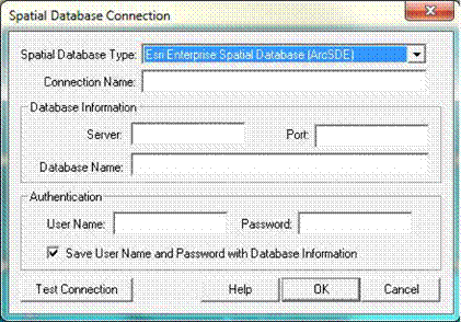
Choose
the option from the Spatial Database Type
drop-down list that corresponds to the spatial database you are using.
Type
a unique Connection Name to identify
this connection. The name you use here will be listed in the connection list on
the Open Spatial Database Dialog.
The
Database Information section
specifies the location of your database on the network. Fields that are not
needed for a particular database vendor will be greyed out and disabled.
• In the Server field, type the name of the
network server where the database is located.
• Specify
the required server port in the Port field.
In an Esri ArcSDE geodatabase connection, this is
also known as the Service parameter.
• Enter the
database name in the Database Name field.
Note that the database name is optional when
defining an Esri ArcSDE geodatabase
connection. Whether or not it is needed is specific to your
particular installation.
Use the Authentication
section to specify the user and password required to log on to the spatial
database.
• Type a
valid User Name.
• Type a
valid Password
• Put a
check next to Save User Name and Password
with Database Information if you want to save the
authentication information along
with the connection definition. The password will be encrypted.
Click
the Test Connection button to determine whether or no the connection
parameters can be used to connect to the spatial database.
Once
you have entered all of the required information, click the OK button to
save the connection definition. The Cancel button quits the process of
creating or updating a connection definition.
The Help button displays the Global Mapper help for this dialog.
5 CHANGE DISPLAY CHARACTERISTICS
Selecting
the [Tools/Configuration] menu item or toolbar button displays the Configuration dialog. This dialog
provides for general setup of Global Mapper display options.
The Configuration dialog
provides the following panels allowing the modification of display options:
• General - Scale, Units, and Position Display Setup
• Vector Display - Vector Display Setup
• Area Styles - Area Type Color/Fill/Border Settings
• Line Styles - Line Type Color/Width/Style Settings
• Point Styles - Point Type Symbol Settings / Custom Symbols
• Vertical - Elevation Display Setup
• Shader - Shader-Specific Setup
 • Projection - Select Display Projection/Datum
General Options
The
General panel (pictured below)
controls options for the display of vector data (areas, lines, and points) as
well as position format on the status bar.

The
Grid Display options allow for the
control of whether or not grid lines are displayed, and if so, what projection
they will be in. The No Grid option
is the default and causes no grid lines to be displayed or exported. The Lat/Lon Grid options causes a grid to be
displayed along even latitude and longitude lines. The Global Projection Grid option causes a grid to be displayed in the
currently selected global (i.e. display) projection, which can be modified on
the Projection tab.
The
Grid Spacing section allows you to specify
whether to allow Global Mapper to automatically determine a good grid spacing
to use or to specify a custom grid spacing.
If
the Show All Grid Lines Regardless of
Zoom Scale option is checked, all grid lines will always be shown rather
than the default behavior of only major grid lines being displayed when zoomed
way out and the more minor grid lines only showing up as you zoom in.
If
the Extend Grid Lines Beyond Loaded Data
Bounds option is checked, the generated grid lines will extend a little bit
beyond the bounds of the loaded data. Otherwise, the grid lines will stop at
the edge of the smallest bounding box encompassing all loaded data files.
If
grid lines are being displayed, the grid lines can also be exported to any of
the supported vector export formats. The color and style of the grid lines can
be modified on the Line Styles tab by
modifying the styles
for
the "Grid Line", "Grid Line - Minor", and "Grid Line -
Major" line types. You can also selectively turn off the display of any or
all of the grid line types using the Filter
options described above.
The
Distance Scale Display options allow
for the control of whether or not a distance scale is displayed on the main map
when data is loaded. The Distance Measure
Units selection below it then controls the units that are displayed on the
scale bar.
The
Elevation Legend Display Units options
allow for the control of whether or not an elevation legend is displayed on the
main map when elevation grid data is loaded and what units the elevation legend
will be in if it is displayed. The No
Legend option causes no elevation legend to be displayed. The Metric (meters) option causes an
elevation legend to be displayed with various elevation values labeled in
meters. The Statute (feet) option
causes an elevation legend to be displayed with various elevation values
labeled in feet. If the elevation legend is displayed in the main map view, you
can right click on it to control various options and also save it
to a BMP file.
The
Position Display Format setting
controls the format of the cursor latitude/longitude position display in the
status bar.
The Area Measure Units
setting controls what units that area measurements will be displayed in the
Measure
Tool and when creating new features with the Digitizer Tool.
The Distance Measure
Units setting controls what units that distance measurements will be
displayed in the
Measure Tool and when creating new features with the
Digitizer Tool as well on on the Distance Scale bar.
The
Miscellaneous Advanced Options section
contains options for advanced users. The following options are available:
• Prefer
World File (TFW) Coordinate for GeoTIFF Files - if checked, this option
specifies that for
GeoTIFF files that also have
accompanying TFW files, the coordinates from the TFW file will be
used rather than the coordinates embedded in the GeoTIFF
file.
• Maintain
Export Bounds Instead of Sample Spacing - if checked, this option
specifies that when
exporting a raster/elevation format
and the bounding box for the export is not an exact multiple of the
specified sample spacing for the export, the sample spacing
will be adjusted to be slightly smaller rather than the default of adjusting
the export bounds up to the next sample spacing boundary.
• Automatically
Anti-Alias Raster Layers When Loaded - if checked, this option
specifies that raster
imagery/scanned map layers will have
bilinear resampling enabled automatically when loaded to
smooth appearance. If not checked then the default nearest
neighbor (i.e. no resampling) option will be used.
• Don't
Automatically Interpolate Terrain Layers on Load - if checked, this option
specifies that
gridded elevation layers will not
have the default bilinear resampling enabled automatically when
loaded to smooth appearance but instead will use the nearest
neighbor (i.e. no resampling) option.
• Use
Current Screen Bounds by Default when Exporting - if checked, this option
specifies that the
default choice on the Export Bounds
tab when exporting should be to use the current screen bounds
rather than exporting all loaded data.
• Default
Contrast Adjustment to Linear Min/Max Stretch - if checked, this option
specified that
layers that come in with automatic
contrast adjustment enabled by default (primarily imagery with
more than 8 bits per color channel) will defualt to using
the linear min/max strecth contrast adjustment mode rather than the standard
deviation adjustment.
• Never
Automatically Contrast Adjust Images on Load - if checked, this option
disables the
automatic contrast adjustment of
imagery with more than 8 bits per color channel on import.
• Minimize
Main Window During Exports - if checked, this option causes the main map window to
automatically be minimized during
most export operations.
• Terrain Export:
Specify Bounds as Pixel is Area - if checked, this option specifies
the the bounding
box that you provide when exporting
to new terrain/ gridded elevation formats will be specifed as
"pixel is area" (i.e. via coordinates of the edges
of the grid cells) rather than the default of "pixel is point" (i.e.
coordinates refer to center of outer grid cells rather than outer edges of
cells).
• BIL
Format: Ask if 16-bit Files are Imagery - if checked, this option
will cause the user to be
prompted to choose whether 16-bit
BIL files that are encountered are elevation or imagery files. If not
checked, any 16-bit BIL files will be assumed to be
elevation files.
• DGN:
Import Cells as Point Features - if checked, this option causes cell
features in DGN v8 and
later files that have an associated
point location to just be loaded as a single point feature rather than
the collection of features specified by the cell.
• DGN: Add
DGN Color Number to Feature Description - if checked, this option
causes the DGN
color number for each feature to be
appended to the feature description/level number.
• DXF/DWG:
Import INSERT entities as point features - if checked, this option
specifies that the
content of INSERT entities (i.e.
blocks) in DXF and DWG files should be loaded as a single point
feature at the location of the INSERT.
• DXF/DWG:
Create New Types from Layers - if checked, this option will cause
new Global
Mapper types to automatically be
created for every DXF/DWG layer name encountered for which a
Global Mapper type does not already exist.
• Show Pixel
Location in Status Bar - if checked, this option causes the native pixel
location of the
topmost raster or gridded elevation
file to be displayed in the status bar as you move the cursor around
in addition to the color and/or elevation data.
• Use DOS
Character Set for Default Label Fonts - if checked, this option
specifies that default
display label fonts should use the
OEM character set (code page 437) rather than the ANSI character
set (code page 1252). This option can be helpful if you are
having problem with accented characters not displaying correctly from some data
sets (those data sets encoded in code page 437 rather than
1252).
• Use Path
to First Loaded File as Default Export Path - if checked, this option specifies
that when
exporting a new file, the default
export path will be the path of the first loaded file during this session
rather than the path to the last exported file in any
session.
• Use CR/LF
in World Files (TFW) Instead of LF - if checked, this specifies
that lines in generated
world files will be terminated using
a carriage return (CR) and linefeed (LF) character as is customary
on Windows systems rather than just a LF character. Use this
if your world files are not being recognized by your Windows-based
applications.
• Automatically
Create Backup Copies of Workspace Files - if checked, this option
will cause your
current workspace file to
automatically be backed up every so often (i.e. after so many vector edits,
etc.). These backup copies will be created in the same
folder as the workspace file and have the suffix
"auto_backupX", where X is a number from 0 to 9.
• Lock
Active Workspace File to Prevent Sharing - if checked, this option
prevents other users from
opening and using the same workspace
file that you are using while you have it open. This is useful in
network environments where you don't want one person's work
to accidentally overwrite anothers. If you try to open a locked workspace, it
will automatically be opened in read-only mode, which will prevent you from
overwriting the original workspace file when saving.
• Don't
Center on Cursor when Zooming with Mouse Wheel - when this option is
unchecked (or
when holding down Ctrl) and you
rotate the mouse wheel over the map, the map will zoom in and out
and maintain the location under your cursor at the same
location rather than just zooming in and out on the current screen center.
• Swap Zoom
Direction Using Mouse Wheel or Hot Keys - when this option is
selected the direction
of zoom when scrolling the mouse
wheel or using the Page Up/Down keys will be reversed.
• Export:
Snap Export Bounds to Pixel Boundary if Possible - when this option is
checked the
bounding box for an export will be
adjusted so that the top left corner of the bounding aligns with the
top left corner of a pixel in the imagery being exported.
This is useful to eliminate any visual sub-pixel shift due to mis-alignment of
the export bounds and the pixels in the input imagery.
• Export:
Keep Pixel if any Part is Inside Crop Area - when this option is
checked and you are
cropping a raster/elevation export
to a selected area feature, an exported pixel/cell will be kept if any
corner of that cell is within the crop area rather than the
default requirement of the center of the cell being in the crop area.
• Disable
Display of Pan Arrows on Map Edge - when this option is checked, the
arrow cursor that
displays near map edges when most
tools are active to allow easy panning are disabled, thus allowing
use of the active tool all the way to the edge of the map
display.
• Always
Display Lat/Lon in Status Bar in WGS84 - when this option is
checked the lat/lon location
displayed on the right side of the
status bar will always be in the WGS84 datum rather than whatever
datum is selected on the Projection tab of the Configuration
dialog.
• Disable
Automatic Interpolation of Resampled Exports - if checked, exported
raster layers will
only be interpolated if the
anti-alias (interpolation) option for that layer is checked, rather than
interpolation occurring for any reprojected or resampled
export.
• Disable
Automatic Interpolation of Zoomed-Out Display - if checked, this option
disables the
automatic
interpolation/anti-aliasing done when zoomed way out on raster/imagery layers.
This can
increase the drawing speed when zoomed out on data, at the
expense of a worse display for most maps.
• Auto-Fake
Location of Unpositioned Rasters - if checked, this options causes the
location of any
un-positioned raster files to
automatically be faked to allow display. This means rather than being
prompted to rectify, fake the position, or cancel the load,
the "fake position" option would just be chosen automatically.
• Export Old
Format PRJ Files - if checked, this option specifies that the old, mostly
unsupported,
ESRI PRJ format be used when PRJ
files are saved rather than the default new WKT projection
format that is used by default.
• Include
Datum Transformations in PRJ Files - if checked, this option
will cause any generated
WKT PRJ files that use a datum based
on a 3-parameter Molodensky or 7-parameter Bursa Wolfe
transformation to include that transformation as a TOWGS84
field in the PRJ file. Note that some products (i.e. ESRI ones) won't accept a
PRJ file with the TOWGS84 field, which is why it isn't always included.
• Create PRJ
Files with .PRJ After Original File Extension - if checked, this option
specified that
any export that generates a PRJ file
will append the .prj to the entire filename rather than replacing the
file extension with .prj. So if you exported a file named
test.ecw with a PRJ file, you would get test.ecw.prj for this export rather
than test.prj.
• Always
Load Duplicate Filenames Rather than Prompting - if checked, you will no
longer be
prompted to abort the load of
already loaded files. The files will just automatically load.
• GeoTIFF
Export: Default to No Compression - if checked, when doing a GeoTIFF
export the
compression will default to 'No
Compression' (if available).
• Don't Copy
Error Text to Windows Clipboard - if checked, text displayed on any
error dialogs will
no longer be automatically copied to
the clipboard as text for pasting. Check this if you are concerned
with text you are working with on the clipboard being
inadvertently erased when a Global Mapper process fails and shows an error.
The Restore Default
Settings button will restore all Global Mapper settings from the
Configuration dialog to their default values.
Vector Display Options
The
Vector Display panel (pictured below)
controls options for the display of vector data (areas, lines, and points).

The
Render section contains the settings
for which types of vector features (areas, lines, or points) are to be
displayed when loaded. You can use these settings to turn off an entire class
of features all at once. For a finer degree of control, see the Filter section described below.
The
Select From section contains the
settings which determine which vector object types (i.e. areas, lines, points)
the Pick Tool will consider when selecting
objects.
The
Filter section allows you to select
which specific area, line, and point feature types you wish to display. By
default, all feature types are displayed.
The
Vector Map Detail setting controls
how much decluttering of displayed vector data is done. This is useful when you
have a large of amount of vector data loaded. For example, if you had all of
the roads for an entire state loaded at once, you could slide the detail slider
to the left to make minor roads been hidden until you zoomed in sufficiently
far on the data. The rightmost (default) setting causes all vector data to be
displayed regardless of zoom scale. This setting does not affect the display of
raster or elevation data sets.
The
Vector Layer Ordering During Draw settings
control the order in which data from vector layers is displayed. The default
setting (order by type before layer order) is that all vector data is drawn
after any other
loaded
raster or elevation data, regardless of how the vector layers are ordered in
the Overlay Control Center. All area
features from all layers will be drawn first, followed by all line features
from all layers, and finally all point features from all layers. Within each
grouping (e.g. areas, lines, or points), the drawing order will be determined
first by type, and then by layer ordering.
The second draw order option (order first by layer, then by
type within a layer) specifies that the order of the vector layers in the Overlay
Control Center should take precedence over all else when drawing. This
means that if a vector layer is before a raster layer in the Overlay
Control Center's draw order, that vector layer will draw underneath that
raster layer if they overlap.
The
Set Default Font Face option allow
you to choose what font face should be used for all feature label displays
where the font has not been explicitly set to something else for the feature.
The Set Default Font
Character Set option allow you to choose what character set should be used
for fonts that are still set to the default for their type. Change this to
allow default display of non-European character sets, like Cyrillic (Russian)
or Japanese.
The
Render Area and Line Vertices option
specifies whether each vertex along area and line features should be displayed
with a large dot.
The
Always Render Vertices for Selected
Features option specifies whether each vertex along area and line features
selected with the Digitizer/Edit Tool should be displayed with a large dot. Use
this option rather than the Render Area
and Line Vertices option above to only display vertices for features that
you are actively editing in order to prevent excessive clutter on the map.
The
Render Dots at Line Endpoints option
specifies whether or not the start and end vertices of line features will be
displayed with a large dot. You can use this instead of the Render Area and Line Vertices option if
you just want to see line endpoints rather than all shape points.
The
Render Deleted Features option specifies
whether or not features that have been deleted by the user should be displayed.
The
Draw Feature Labels option specifies
turns labeling of features on or off globally. For more fine-grained control
over which types are labeled, check the Area
Styles, Line Styles, or Point Styles tab.
The
Always Display All Labels option
specifies whether or not feature labels should be allowed to overlap when
drawing them on the screen. When this option is not checked (this is the
default), labels that collide with other labels on the screen will be discarded
until you zoom far enough in on the feature so that they can be displayed
without overlapping any other labels.
The
Render Segment Lengths on Map option
specifies that when you zoom in on line features that the length of each
segment should be displayed on the map along the segment.
The
Render Segment Bearings on Map option
specifies that when you zoom in on line features that the bearing of each
segment should be displayed on the map along the segment.
The
Render Line Direction Arrow option
specifies whether or not a small arrow should be drawn on each line feature
indicating in which direction the line vertices go. The arrow will point along
the line towards the last vertex in the line.
The
Hide Extra Label Text Displayed Under
Road Icons option allows you to control whether or not any extra text
displayed below road icons, like alternate names for the road, are displayed.
The Only Highlight
Border of Selected Area Features option allows you to change the rendering
style for area features selected with the Feature Info or Digitizer Tools so
that only the border of the area is highlighted and the center is left
unfilled.
The
Mark Sides of Road with Addressing
Information option allows you to have the sides of roads with recognized
address numbering information to be marked with a series of parallel lines
extending from the road on the side(s) with known address information. This
provides a visual way to see where addressing
information is available.
The Hide Display
Labels that are Partially Offscreen option allows you to hide any feature
labels that don't entirely fit on the screen. This can be useful when exporting
vector data to a raster format and also gridding the export into multiple
pieces. This option should allow a seamless result in that case.
The Add MODIFIED_DATE
to Modified Vector Features option controls whether or not a
MODIFIED_DATE attribute is automatically added to vector
features when they are changed in some way.
The
Iconize Road Names on Import (Some
Formats) option controls whether or not the specified name for road line
types is checked on import to see if it should result in an iconized road name
display (such as for interstates and major highways). This is only done for
formats which do not already have their own built-in iconization (such as
Tiger/Line and USGS DLG files). For example, this will work for formats like
Shapefiles and MapInfo MIF/MID files (among others).
The
Fix Line Label Position on Longest Segment
option controls whether or not the label displayed for line features should
move around to always be centered on the longest on-screen segment (the default
unchecked behavior) or should remain fixed on the center of the longest segment
of the line, regardless of whether it is
on-screen
or not. Checking this can prevent your line labels from jumping around as you
zoom in and out, but can result in a lot of unlabeled lines if you zoom in too
far.
The
Only Snap to Area and Line Vertices by
Default option controls whether or not the snapping
behavior of the Digitizer Tool will
snap to anywhere on existing area and line vertices (the default unchecked
behavior) or will only snap to vertices on area and line features. Holding down
the 'V' key when drawing will toggle this behavior.
The
Only Display Area Labels when Completely
Inside Area option allows you to easily disable the display of any area
label when that label is not completely contained within the area feature that
it is labeling. This is useful to keep area labels from displaying until you
are zoomed in far enough on the area for a label to be appropriate.
The Don't Add Measure
Attributes to New Features option allows you to disable the automatic
adding of measure attributes, like LENGTH, PERIMETER, ENCLOSED_AREA, etc. to
new area and line features created with the Digitizer Tool.
The
Make Duplicate Vertex Turn Off Area
Border Segment allows you to use duplicate area vertices to turn segments
of the area border on and off. This is known as Pen Up/Pen Down display. How it
works is that the border pen is on (down) at the start of the border. Whenver a
duplicate vertex is encountered, then pen it turned off for the next segment.
So if for example you had vertex 1, then a duplicate vertex 2 and 3, then
non-duplicate
vertices 4 and 5, you would get a border drawn from vertex 1 to vertex 2, then
it would turn off for 3-4, then be drawn again for 4 onto the end.
The
Disable Snapping to Features in the
Digitizer Tool option allows you to disable automatic snapping to nearby
features when drawing in the Digitizer Tool. If you check this option then
snapping will be disabled by default and holding down the ALT key can be used
to enable snapping (the default behavior is the reverse).
The Snap to Grid Lines
if Displayed option allows you to disable automatic snapping to nearby grid
lines features when drawing in the Digitizer Tool. If you check this option
then snapping to grid lines will be disabled.
Area Styles
REFERENCE GUIDE ALERT!
Built-In Area Types and Styles - A graphical reference guide to the area types and
border/fill styles built-in to
Global Mapper.
The
Area Styles panel (pictured below)
allows the user to configure how areas of a given type will be displayed in
Global Mapper. The area fill and border style and color can be modified on a
type-by-type basis. You can also use the Add
Custom Fill Pattern option to provide your own image to use as a fill
pattern. For transparent or translucent patterns, use a transparent PNG format
image file when creating the custom fill pattern.
With
the Transparency slider users can make solid filled areas partially see-through
(translucent) in order to see data underneath the area. In addition, the Show Labels for Areas of This Type When
Present option allows users to turn area labels off on a type-by-type
basis.
The
New Type button allows the user to
create a new area feature type and specify how it should be displayed. The Edit Type button allows the user to edit
area types that were previously created with the New Type button, and the Delete
Type button allows the user to remove area types that were previously
created with the New Type button.
With the Attributes button you can
specify a set of default attributes and values to use for new features of this
type created using the Digitizer Tool.
If
you right click on the list of types, a menu will appear allowing you to save
and restore your style settings using a style file. This provides an easy way
to setup a set of styles to use, then restore them at a later date for use with
a particular set of data.

Line Styles
REFERENCE GUIDE ALERT!
Built-In Line Types and Styles - A graphical reference guide to the line types and drawing
styles built-in to
Global Mapper.
The
Line Styles panel (pictured below)
allows the user to configure how lines of a given type will be displayed in
Global Mapper. The line style, width, color, and label font can be modified on
a type-by-type basis. When selecting a line width, you can choose a fixed width
in screen pixels, which means that the line will draw the same width regardless
of your zoom level, or you can choose the option to specify the line width as a
New Fixed Width in Meters. When you
do that your line will be drawn at a given number of meters in width, which
means it will get thicker as you zoom in and smaller as you zoom out to
maintain the same width in ground units.
In
addition, the Show Labels for Lines of
This Type When Present option allows users to turn line labels off on a
type-by-type basis. The Display Roads As
Fat Lines When Zoomed In option allows users to turn on/off the
"fattening" of road lines when zoom in tight on them.
The
New Type button allows the user to
create a new line feature type and specify how it should be displayed. The Edit Type button allows the user to edit
line types that were previously created with the New Type button, and the Delete
Type button allows the user to remove line types that were previously
created with the New Type button.
With the Attributes button you can
specify a set of default attributes and values to use for new features of this
type created using the Digitizer Tool.
If
you right click on the list of types, a menu will appear allowing you to save
and restore your style settings using a style file. This provides an easy way
to setup a set of styles to use, then restore them at a later date for use with
a particular set of data.

Point Styles
REFERENCE GUIDE ALERT!
Built-In Point Types and Symbols - A graphical reference guide to the point types and
symbols built-in to
Global Mapper.
The
Point Styles panel (pictured below)
allows the user to configure what symbol will be used to display points of a
given type and at what angle, if any, to rotate the symbol when displaying it
on the map. Symbols can be rotated relative to either the map display (where 0
degrees is always straight up) or relative to true north, where 0 degrees
always points directly to the North Pole. Rotated symbols are good for use in
geology maps and for adding things like north arrows to your maps.
You
can also press the Scale button to
scale a point symbol to make it larger or smaller. For example, to double the
size of a symbol use a scale of 2.0, whereas to make a symbol half its original
size, use a scale of
0.5.
You can also specify a symbol size in meters. This will automatically scale the
point so that it is always the specified number of meters tall on the map
regardless of zoom level.
The
symbol selection list also includes several option at the top of the list to
select symbols of common shapes, like dots, squares, diamonds, etc. with a
user-specified size and color.
In
addition, the Show Labels for Points of
This Type When Present option allows user to turn point labels off on a
type-by-type basis. The Custom Symbols section
allows users to create new symbols from their own bitmap and icon files which
they can then use as the symbol to display for a given type.
The
New Type button allows the user to
create a new point feature type and specify how it should be displayed. The Edit Type button allows the user to edit
point types that were previously created with the New Type button, and the Delete
Type button allows the user to remove point types that were previously
created with the New Type button.
With the Attributes button you can
specify a set of default attributes and values to use for new features of this
type created using the Digitizer Tool.
If
you right click on the list of types, a menu will appear allowing you to save
and restore your style settings using a style file. This provides an easy way
to setup a set of styles to use, then restore them at a later date for use with
a particular set of data.
The
Custom Symbols section allows you to
add new point symbols that will be available for display from your own files.
This includes support for transparent symbols from PNG, ICO, GIF, and 32-bit
alpha BMP files, as well as symbols from JPG images. You can also add vector
symbols from EMF, DXF and GM_SYM (Global Mapper Symbol) files. GM_SYM files are
simply ASCII text files that the File->Open Generic ASCII Data File menu
command couuld load, with 0,0 being the center of the symbol and the
coordinates specified as pixels, with X increasing to the right and Y
increasing to the top of the symbol. Vector symbols will scale much more
cleanly than symbols based on images.

If
you press the Select Label Font... button,
the font selection dialog (pictured below) for the selected point type will
appear. This dialog allows you to select the font to use for the point, as well
as set up other label display options for the point, including where to
position the label relative to the point, what angle (if any) to rotate point
labels at, how to fill the background for the labels, and whether or not to
display the labels at a fixed height in ground units rather than a fixed font
size in pixels.

Vertical Options
The Vertical Options panel
(pictured below) controls options for the display of elevation data.
The
Shader selection box allows for the
selection of the algorithm used to color and shade any loaded elevation data.
The following shading algorithms are available:
• The Atlas
Shader is the default shader. It generally provides good results for any
loaded elevation
data.
• The Color
Ramp Shader displays ramps color from blue for low elevations to red for
the highest
elevations by default.
• The Daylight
Shader colors all elevations the same and is only useful when hill shading
is turned on.
• The Global
Shader is designed for shading elevation data sets covering large areas of
the earth such
as Terrain Base and GTOPO30. The
results are quite stunning for data sets such as these.
• The Gradient
Shader moderates the color with elevation between the low elevation and the
high
elevation. The actual colors ramped
between can be selected on the Shader Options
panel.
• The HSV
Shader maps the elevations onto the HSV (hue saturation value) color space.
The mapping
can be configured on the Shader Options panel.
• The Slope
Shader colors loaded terrain data by the slope of the terrain rather than
the absolute
elevation. This shader allows you to
identify the portions of the terrain that are relatively flat vs those
that are relatively steep. The definitions of
"flat" and "steep" are user configurable on the Shader
Options panel.
• The Slope
Direction Shader colors loaded terrain data by direction in which the
terrain faces rather
than the absolute elevation. This shader allows you to
easily identify things like the portions of the terrain that face south, or any
other direction. The colors to use for each direction are user configurable on
the Shader Options panel.
• If any custom shaders have been
created, they will be available as well.
Use
the Enable Hill Shading option to
view elevation data as shaded relief. With this option off, the map appears
flat, with elevations distinguished by color only. With it on, shadows are
generated using the loaded elevation data along with the remaining settings on
this panel.
The
Elevation Display Units option allows
you to modify the units that elevations will be displayed in on the status bar
as you move the cursor over loaded elevation data.
The
Lighting Direction options set the
position of the light source (the "sun") for performing hill shading.
Note that cartographic azimuth and altitude are used. This means that 0 azimuth
means the sun is to the north,
90
azimuth means the sun is to the east, and so on. An altitude of 90 means that
the sun is directly overhead, while an altitude of 0 means the sun is on the
horizon.
Use
the Ambient Lighting to brighten up
dark looking data sets or dim bright looking data sets. The Vertical Exaggeration setting is used to
control the exaggeration of relief features.
The
Hill Shading Shadow Darkness setting
is used to control how dark that hill shading is allowed to make shaded areas.
By default, the value of 0 allows shaded areas to go all the way to black. By moving
this slider to the right you can cause shadowing to be capped in high relief
areas, thus allowing the use of other controls to better bring out detail in
low-relief areas.
The Hill Shading
Highlight from Direct Light setting is used to display a whitened highlight
area in terrain areas that are getting direct sunlight based on the lighting
angle selected. The slider controls the amount of whitening highlight applied
to those direct sunlight areas.
To enable the display of water on elevation data sets, check
the Show Water On Elevation Data option.
The
Water Transparency controls the
clarity of displayed water if configured to display water. Clearer water shows
more underlying relief to show through, while opaque water allows none.
The
Water Level setting controls the
level at which water is displayed. The default is set at an elevation of 0
meters above sea level. Use this to simulate different flood and sea level
change scenarios.
The Water Color options
allows you to set the color of the water. The default is blue. Shader Options
The Shader Options panel (pictured below) controls options for the
display of elevation data using the
daylight, gradient, slope, and HSV shaders (described
above).

Daylight Shader
• Surface Color: Sets the calculated surface
intensity color.
Gradient Shader
• Low Color: Sets the lowest elevation value
color.
• High Color: Sets lowest elevation range color.
Slope Shader
• Minimum Slope -> Slope Value: Allows
the user to set the slope at or below which the Minimum
Slope Color is used.
• Minimum Slope -> Color: Specifies the color which
all parts of the terrain with a slope at or below the
Minimum Slope Value will be colored
with.
• Maximum Slope -> Slope Value: Allows
the user to set the slope at or above which the Maximum
Slope Color is used.
• Maximum Slope -> Color: Specifies the color which
all parts of the terrain with a slope at or above
the Maximum Slope Value will be
colored with.
• Smooth Gradient: Specifies that all portions
of the terrain with a slope between the Minimum Slope
Value and the Maximum Slope Value
will be colored with a smooth gradient of colors that vary with
the slope from the Minimum Slope Color to the Maximum Slope
Color.
• Custom Color: Specifies that all portions of the
terrain with a slope between the Minimum Slope
Value and the Maximum Slope Value
will be colored with a single color that can be modified with the
Select... button.
Slope Direction Shader
• East Color: Allows the user to set the color to
use for slopes facing directly East.
• North Color: Allows the user to set the color to
use for slopes facing directly North.
• South Color: Allows the user to set the color to
use for slopes facing directly South.
• West Color: Allows the user to set the color to
use for slopes facing directly West.
• Angle Offset: Allows the user to specify an angle
offset in degrees to add to the calculated slope
direction
in order to shade against slope directions other than cardinal directions.
HSV Shader
• Low Color Start (Advanced): Sets where in
the HSV color range the lowest elevation will be.
• Value (Advanced): Modifies the HSV value
parameter.
• Saturation (Advanced): Modifies the HSV
saturation parameter.
• Range: Modifies how much of the full HSV range is to be used.
Increasing this value leads to color
wraparound.
Custom Shaders
The Custom Shaders section
allows the user to manage any custom shaders that they may have. Custom shaders
allow the user to control exactly how elevation data is rendered so that the
desired result can be obtained.
Pressing
the New... button displays the Custom Shader dialog (pictured below)
which allows the user to create a new custom shader. Pressing the Edit button display the same dialog,
allowing the user to edit the currently selected custom shader. The Delete button removes the currently
selected custom shader.

The
Custom Shader dialog allows the user
to specify how they want elevation data to be rendered. The Name field provides a place to enter the
name to associate with the shader to allow the user to select it. The Elevation Colors section display the
elevations and their color values associated with the custom shader. Pressing
the Change Color and Change Elevation buttons allow the user
to change the values associated with the current elevation selected in the Elevation Colors list. The Delete Elevation button allows the user
to
delete
the currently selected elevation. New elevations can be added by entering the
elevation (in the currently selected units) and pressing the Add button.
The
Evenly Space Elevations Starting at
Arbitrary Base Elevation button will allow you to quickly populate the list
of elevation values with a series of evenly spaced values starting at some
specified elevation. You can then assign the colors as desired after that. For
example, you could use this to quickly populate the list with all elevations
from 0 meters to 5000 meters with an elevation every 500 meters, then modify
those as desired.
The
Initialize from Other Shader button
will allow you to initialize the list of color/elevation pairs to those used by
either the Global Shader built into Global Mapper or another user-created
custom shader. This allows users to easily create a slightly modified version
of an existing shader if they'd like.
The
Initialize from Palette File button
allows you to initialize the list of color/elevation pairs from a color palette
file in any recognized format (like a comma-delimited file of R,G,B components
on each line). Since palette files don't contain elevation values, the
elevations will be incremented by one for each color and set to automatically
scale the colors between loaded elevation values.
The Initialize from
Surfer CLR File button allows you to initialize the list of color/elevation
pairs with a a CLR file created by the Surfer application by Golden Software. You can use the Save
to Surfer CLR File button to save your custom shader to a CLR file. This is
useful for making copies of a custom shader and
providing them to other users.
Elevations
shaded with a custom shader will use the color specified for each elevation
value. Any elevation values between two elevation/color values will be a blend of
the two bounding colors if the Blend
Colors Between Elevation/Slope Values option is checked. For example, if an
elevation of 500 meters was set to black and an elevation of 1000 meters was
set to white, an elevation of 750 meters would be colored a medium shade of
gray. Any elevations below the minimum specified elevation will use the same
color as the minimum elevation. The reverse is true for any elevations over the
maximum elevation. If the blend colors option is not checked, any elevation
between two elevation values will be set to the color associated with the lower
of the elevation values.
If
you would like the elevation values selected to scale to the elevation range of
the currently loaded data rather than stay at fixed elevation values, check the
Scale Shader to Loaded Elevation Values.
This will make your shader behave similar to most of the built-in shaders, like
the Atlas or Color Ramp shaders. For example, if you check this option and
specify that an elevation of 0 meters is blue and 1 meter is red, and the
actual loaded data has a range of 100 meters to 500 meters, then 100 meters
will be blue and 500 meters will be red, with the values gradually shaded in
between (if you have the blend colors option checked).
If you would like to shade based on the slope of the terrain
rather than the elevation values, use the Shade
Slope Values (Degrees) Rather than Elevations option. This will change the
provided values so they are treated as slope angles in degrees and allow you to
setup shading based on the slope.
Projection
The
Projection panel (pictured below) is
used to modify the projection and datum that the currently loaded data is
displayed in.

Use
the Projection pull-down menu to
select the projection you wish to view the currently loaded data in. The Geographic
projection is really the absence of a projection. It is just a linear
mapping of latitude/longitude to a grid. For a good description of most of the
other supported projection systems and a discussion of the tradeoffs in using
various projections, we suggest visiting http://www.progonos.com/furuti/MapProj/Normal/TOC/cartTOC.html.
The
Datum pull-down is used to select the
datum to use in association with the projection. The most commonly used datums
are WGS84, NAD27, and NAD83. If you find that the datum that you need is not
available, you can use the Add Datum button
to add your datum. When that button is pressed, the Create New Datum dialog (pictured below) is shown, allowing you to
enter the parameters for either a 3-parameter Molodensky datum transformation
or a 7-parameter Bursa-Wolfe datum transformation, or even specify a
transformation defined by a text file with a list of control points.
If
you choose the Custom Shift Based on
Control Point File option, the text file that you select should have a
series of lines defining the mapping from a lat/lon coordinate in the new datum
and the corresponding lat/lon value in WGS84. This is a very easy way to define
a datum if you don't know any transformation parameters, but do know the WGS84
coordinates for at least 2 coordinates in the new datum. The format of each
line would be as follows:
deg_longitude_in_new_datum,deg_latitude_in_new_datum,deg_longitude_in_WGS84,deg_latitude_in_WGS
The
Abbreviation field is what will be
displayed for the datum name in the status bar. If your datum uses a prime
meridian other than Greenwich, enter the longitude of the meridian used (relative
to Greenwich) in the Prime Meridian entry
box.
The
datum information will be stored in the custom_datums.txt file in the Global
Mapper Application Data folder (see the Help->About dialog for the location
of this folder), so to share your datums just copy that file to that folder on
another user's computer. If a needed ellipsoid is not built in to Global
Mapper, use the Add Ellipsoid button
to add a new one or Edit Ellipsoid to
edit an existing custom ellipsoid definition.

The Planar Units pull-down
select the ground units to use with the projection.
The
Zone selection allows you to select
the zone for use with the UTM, State Plane, Gauss Krueger,
and other zoned projections.
For
those projections that require additional parameters to fully define them, the Attributes table allows you to enter the
values for each applicable parameter.
You
can save the currently selected projection to a PRJ file using the Save to File button. Previously saved
PRJ files can be loaded using the Load
from File button. By default, the PRJ file will be saved in the newer WKT
(well-known-text) format used by most products. There is an Advanced Option on
the General tab of the Configuration dialog allowing the older ESRI PRJ format
to be exported instead if you would like. If for some reason a
WKT-representation of the projection cannot be generated, the old ESRI PRJ
format will be written out instead.
The
Init From EPSG button allows you to
initialize a projection definition based on a numeric EPSG projected coordinate
system definition. There are numerous built-in EPSG code definitions, but by no
means is there an exhaustive set. You can add your own EPSG code definitions
(or modify built-in ones) by modifying the epsg_codes.txt file installed in your
Global Mapper installation folder. The format is described in the file header.
You must re-start Global Mapper after changing this file for the changes to
have any effect.
OVERLAY CONTROL CENTER
This
section describes the Overlay Control Center dialog (pictured below). This
dialog serves as the central control center handling all currently loaded data
sets (overlays).

Currently Opened Overlays
This
is a list of the all currently opened overlays. You can select an overlay by clicking
on its name. Multiple overlays can be selected using the shift and control keys
while clicking on overlays in the list. If the overlay is currently hidden, it
is indicated to the left of the overlay description. Double-clicking on a layer
automatically brings up its Options dialog. If you hold down the 'M' key while
double-clicking the Metadata dialog for the layer will be displayed instead.
You
can right click on the list of currently opened overlays to display a list of
options available to perform on the selected overlays. Examples of available
options include the following:
• Create
Elevation Grid from 3D Vector Data - This allows you to create an elevation
grid from part or
all of any vector features in the
selected overlays that contain elevation data.
• Modify Image Position - This allows you to reposition imagery and
vector data that was not correctly
positioned when loaded, including
imagery that was manually rectified. See the option below if you
just want to shift an entire layer by some distance.
• Setup What
Zoom Levels to Display Selected Layer(s) At - This option allows you to control
what
zoom levels/scales that the selected
layer(s) will display at. You can choose to have layers only
display below a certain zoom scale or between scales, or
when the map is a certain percentage of the map display size or the map
resolution reaches a certain level. If you choose to show when the map covers a
certain percentage, if the upper range is 0 the map will always show above the
bottom range. Otherwise it will show between the specified ranges.
• Shift
Selected Layer(s) a Fixed Distance or Transform Coordinates - This option
provides a quick
way to shift any layer some fixed
distance in any direction or to shift layers based on a transformation
described in a control point file or via a transformation
dialog. When selected a dialog is presented allowing you to select the type of
transformation to perform. The following options are available:
♦ Shift
Layers a Fixed Distance - presents a dialog allowing you to specify the
distance to shift
the
selected layers in the X and Y direction or some distance along a particular
bearing.
♦ Transform
Coordinates Based on File - you will be prompted to select a control point file
describing a transformation from the
current coordinate system of the file to some new
coordinate locations. The file should be a simple
comma-delimited text file with each line describing a transformation as
follows: current_x,current_y,new_x,new_y. There must be at least 2
transformation lines specified.
♦ Specify
Coordinate Transformation - allows you to specify a generic coordinate
transformation with an offset,
scale, and rotation about some point. The information provided
should be in the same coordinate system (projection) as
natively used by the layer(s) being transformed. You can save the coordinate
transformation that you define to a .gm_xform file. If that file is saved
alongside a vector file and has the same name (i.e. my_file.gm_xform in the
same folder as my_file.dxf), then that transformation will automatically be
loaded and applied to the coordinates in the file.
• Scale
Layer Based on Actual Length of Selected Line - This option allows you to scale
a selected
layer based on a user-specified
length of a selected line feature in that layer. This is useful if you
know the actual length of a line feature in a vector layer
and want to scale the layer so that the line length is correct without caring
about where on the earth the layer is placed. The line that you know the length
of should be selected with either the Feature Info or Digitizer Tool.
• Create
Workspace File from Selected Layer(s) - This option allows you to generate a
workspace just
containing the selected layer(s) and
their display options. This workspace can later be loaded with the
File->Load Workspace menu command.
• Create Map
Catalog from Selected Layer(s) - This option allows you to generate a map
catalog file
containing the selected layer(s).
This map catalog can later be loaded with the File->Open Data File
menu command.
• ROUGHNESS
- Create Roughness Grid from Land Cover Layer - This option allows you to
generate
a grid (and optionally areas) of
roughness length values from a land cover layer. When you select this
option, the following dialog appears allowing you to setup
the roughness calculation:

The
roughness grid is useful for wind power applications and can be exported to a
WindSim GWS file as a roughness layer or the roughness areas can be exported to
a WaSP .map file. Several land cover data sets useful for roughness length
calculation, like CORINE, NLCD, and VCF, have built-in roughness conversion
tables available. Custom roughness tables can be defined in a
roughness_tables.txt file in the settings file path listed on the Help->About
dialog. A sample roughness_tables.txt file can be found here.
• Zoom to
Selected Layer(s) - This causes the view to be zoomed such that the full
extents of the
selected overlays are visible.
• Zoom to
Full Detail For Layer - This causes the view to be zoomed such that a single
sample/pixel in
the selected overlay will take up
approximately one pixel on the screen.
• Set Group
to Assign to Selected Layer(s) - This allows you to specify a group to assign
the selected
layer(s) to. If layers are in a
group, they will be organized under that group name in the Control
Center and you can easiliy collapse them into a single item
in the list of layers and operate on all items in the group by selecting the
parent group item.
• Create
Area Features From Selected Layer Bounds - This causes new rectangular area
features with
the name of the overlay as the
display label to be created for each selected layer in the User-Created
Features Layer. This is useful for creating an image index
as the filename of the layer will also be saved as an attribute of the area
feature created from it.
• GRID -
Create Point Features at Elevation Grid Cell Centers - This causes a new layer
to be created
for each selected elevation grid
layer with a spot elevation point feature at each grid cell center
location. This provides a handy way to edit elevation layers
as you can edit the elevation attribute of the created points or remove bad
points, then create a new elevation grid from the layer.
• CALC ATTR
- Calculate/Copy Attribute Value - This allows you to create a new attribute
value (or
update an existing one) by copying
the value of some attribute, performing a mathematical operation
either between two attributes or an attribute and some
number, or to append some text string to a value. The dialog below is displayed
when you select this option to allow you to set it up:
• JOIN TABLE - Join Attribute Table to
Data Set - This allows you to join a table of attribute values, either from a
DBF file or from a text file, to the attribute table of a selected layer based
on a common value of some attribute. You will be prompted to select the
attribute from the attribute table file to join against a user-selected
attribute from the selected layers. For text files, the first line must contain
the attribute/column names. Whenever a match is found, the other attributes
from the data table are added
to the matching record(s) in the file.
• DENSITY -
Create Density Grid - This causes a new layer to be created by calculating
density values
from the point features in the
selected layer. You can setup the density grid to be based on a simple
point count or as a sum of the numeric values of some
attribute value for the points within some search radius. The Density Grid Setup
dialog (pictured below) appears when you select this option, allowing you to
control the density grid calculation.

The Population Field option
allows you to control whether a simple point count or attribute value is used
to compute the density grid. The Search
Radius option allows you to specify how far from a grid sample location a
point can be and still be considered as part of the value. The Density Type option allows you to
specify whether a weighted-distance Gaussian distribution is used (this gives
much prettier results) or a simple in-or-out of radius calculation is used. The
Shader option allows you to control
which elevation shader is used to render the computed grid. You will often want
to select a specific shader rather than using the default shared one as the
data won't typically render well with other loaded grid layers.
• Create
Area Features from Equal Values in Selected Layer - When a single raster or
elevation grid
layer is selected (with the
exception of online sources), this option appears and allows you to create
area features covering each distinct color or elevation
value encountered in the raster file. This is useful for automatically creating
areas for things like land cover raster files in a vector format.
• Find
Extreme (Min/Max) Elevation Values in Selected Layer(s) - This scans the
selected elevation
grid layers to find the minimum and
maximum elevation values and reports both the values and their
locations to the user. The complete list (up to 10,000
shared location) will be saved to a file, and a shorter list presented to the
user.
• Change
View Shed Layer Color - This allows you to edit the color used to display the
coverage area
for a selected view shed layer.
• Edit View
Shed Parameters and Recalculate - This allows you to edit the calculation
parameters for a
view shed layer and then update the
results.
• Open
Selected Map Folder in Windows Explorer - This causes the Windows Explorer
application to
be opened to the folder containing
the selected map file.
• Split Into
Separate Layers Based on Description/Attribute Value - This option allows you
to create
new layers by splitting the selected
layer(s) into new layers based on a particular attribute value or by
the description, type, or name of each feature. The new
layers will be grouped together using the name of the original layer unless the
original layer was already in a group.
• Allow
Feature Selection from Selected Layer(s) - This option controls whether or not
vector features
from this layer can be selected
using either the Feature Info or Digitizer Tools.
• Select All
Features in Selected Layer(s) with Digitizer Tool - This option causes all
features in the
selected layer(s) to be selected
with the Digitizer Tool.
• Close All
Hidden Layers - This option causes all layers that are currently marked as
hidden (i.e. have
their display checkbox unchecked) to
be closed.
• Hide All
Offscreen Layers - This option causes all layers that are currently completely
off of the main
map view to be marked as hidden (i.e.
have their display checkbox unchecked).
• Remove All
Onscreen Layers from Map Catalog - This option appears when you right-click on
a map
catalog layer and allows you to
remove all of the maps from the map catalog whose bounds intersect
the current screen bounds. If multiple maps are onscreen you
will be presented with a list of those
maps so you can control which ones to remove.
• Hide
Layers that Outside Selected Area Feature(s) - This option causes all layers
whose bounds don't
intersect the currently selected
area feature(s) to be marked as hidden. The area(s) need to be selected
with the Digitizer or Feature Info tools.
• Reorder
Maps by Resolution/Description/Location - This option displays a dialog
allowing you to
choose a method by which to reorder
the maps in the list. This includes sorting alphabetically, by
resolution, or spatially sorting the maps.
• Move
Selected Overlay(s) Up/Down - These options allow you to modify the order in
which overlays
are displayed in the main view. The
large arrow buttons on the right-hand side of the dialog also
perform these functions.
Create Elevation Grid from 3D Vector Data
Selecting
the Create Elevation Grid from 3D Vector
Data option on the popup menu that appears when right-clicking on vector
layers in the Overlay Control Center displays the Elevation Grid Creation Options dialog, pictured below. Using this
dialog, you can configure how you want the elevation grid to be created using
the selected vector data as well as what portion of the selected overlays to
use when creating the elevation grid. You can also use the Gridding tab to specify that your data should be gridded in
sections. This makes it possible to grid data sets that are too large to grid
all at once.
The following options are also available when generating the
grid:
• Use 3D
Line Features as Constraints (i.e. Breaklines) - If this option is checked, any
line and area
features that have elevation values
associated with them will be treated as constraints/breaklines. This
will ensure that elevation values along the line/area
boundary will be consistent with the elevation that should be along the line.
• Flatten 3D
Area Features - If you have any area/polygon features with elevation in the
selected layers
that you are gridding, they will be
treated as flattened areas rather than just additional 3D data
points/constraints. This allows you to create flattened
areas like lakes and also nice terrain surfaces from things like building
models. If only 3D area features are present, any grid locations outside of the
areas will be marked as invalid, otherwise the grid locations within areas will
just be flattened to the area heights and the remainder of the grid will be
generated as usual.
• Taper 3D
Area Features Using Curve Value - If you have any area/polygon features with
elevation in
the selected layers that you are
gridding and you also checked the option to flatten 3D area features,
the taper option allows you to specify that rather than
making the areas absolutely flat, the edges should be tapered with the area
elevation existing near the centroid of the area and the elevation
applied for the area dwindling to zero as you reach the area
edge. The curve value specifies the exponent to apply to the percent distance a
sample location is between the area centroid and the area edge to adjust the
height applied at that location. Values less than 1 will make the edge
steepness progressively greater (i.e. flatter at the middle, then steep edges),
while values larger than one cause the steepness to be near the area centroid
and flatter towards the edges, while a value of 1 provides for a linear taper.
For example if you want to simulate a sand bunker for a golf course, a value of
around
0.5 provides a decent simulation of a bunker.
• Ignore
Zero Elevations - If checked, this option will cause any features with an
elevation value of zero
to be ignored. This is useful if you
have a data set where features with no known elevation are marked
with an elevation of zero.
• Save
Triangulated Network (TIN) as a Vector Layer - If checked, this option will
cause a separate
vector layer with area features for
each 3D triangle created as part of the triangulation and gridding
process. This is known as the TIN surface.
• Heights
Relative to Ground - If you check this option, all elevation values from the
selected vector
layers will be treated as relative
to the height of any loaded underlying terrain surface (like a DEM).
This is very handy for doing things like creating building
models where you just know the building height above ground and not above sea
level.
• Fill
Entire Bounding Box Instead of Just Inside Convex Hull - If you check this
option, the generated
elevation grid will contain valid
values filling the entire bounding box specified for the gridding
operation. Otherwise, the valid values will only fill out to
the convex hull polygon of the data being gridded.
• Export
Grids Directly to Global Mapper Grid Files - If checked, this option will cause
the generated
elevation grid file(s) to be
directly exported to Global Mapper Grid (GMG) files. This is useful when
you are triangulating and gridding a very large collection
of data and also using the Gridding tab to split the operation into smaller
pieces. By directly exporting the results to GMG files you can create elevation
grids that normally would not all fit into memory.
Metadata
Pressing
the Metadata... button displays
metadata for the selected overlay. The actual metadata dialog displayed depends
on the type of the selected overlay. The metadata dialog for a SDTS DLG is
shown below.

Options
Pressing
the Options... button displays a
dialog containing the available display options for the selected overlay(s).
Options can be set on multiple raster or elevation overlays at the same time.
The available display options depend on the type of the selected overlays. The
following display options are used:
• Vector Data Options
♦ Feature Types/Labels/Elevations Tab
♦ Area Styles Tab
♦ Line Styles Tab
♦ Point Styles Tab
♦ Projection Tab
• Raster Data Options
♦ Display Tab
♦ Color/Contrast Adjustment Tab
♦ Cropping Tab
♦ Band Setup Tab
♦ Palette Tab
♦ Feathering Tab
♦ Color Grade Tab
• Elevation Data Options
♦ Display Tab
♦ Alter Elevation Values Tab
♦ Feathering Tab
Vector Data Options
Selecting the Options...
button while a vector (i.e. SHP, DXF, E00, etc) overlay is selected
displays the Vector
 Options dialog (pictured below). Feature
Types/Labels/Elevations Tab
Options dialog (pictured below). Feature
Types/Labels/Elevations Tab
The
Feature Types/Labels/Elevations tab
provides the ability to specify which attribute field(s) (if any) to display as
the name of features loaded from the vector file. You can choose from the
following options:
• Don't Use
an Attribute Value for Name - this option specifies that the
original or edited display
label associated with a feature
should be used for display and not a label based on an attribute value or
custom string
• Use
Selected Attribute Value for Name - specifies that the value of the
selected attribute will be
used as the display label for the
feature. If the feature already had a label and the Keep Original Label
if Non-Empty option is checked, the original label will be used rather
than the attribute value.
• Use
Multiple Attributes for Name - allows you to choose one or more
attributes to combine to
create the display label, as well as
provide custom prefix, suffix, and separator strings. If the feature
already had a label and the Keep Original Label if Non-Empty option is checked, the original
label will be used rather than the attribute value.
• Use Custom
Formatting String for Name - allows you to provide a custom formatted string that
can
contain any free-form text and
attribute values embedded as %ATTR_NAME%. You can use the
name of any feature attribute as ATTR_NAME or special
attributes, like <Feature Name>, <Feature Desc>, <Feature Layer
Name>, etc. For example, to create a display label from the original feature
label, the layer name, and an attribute named FCODE, you could use the
following: %<Feature Name>% - Layer Name: %<Feature Layer Name>% -
Feature Code: %FCODE%. If the feature already had a label and the Keep Original Label if Non-Empty option
is checked, the original label will be used rather than the attribute value.
You
can also select which attribute field (if any) to use for the
"elevation" value for the layer. By default, several attribute field
names (like "ELEVATION", "ELEV", "ALTITUDE",
"Z", etc.) are checked when an elevation value for the feature is
needed. This option allows you to override this behavior and manually select
the attribute to use. You can also select what units to assign to unspecified
elevation values for the layer, such as per-vertex elevation values for 3D line
and area features in the layer. Finally, there are also options available to
select the classification to apply to unclassified area, line, and/or point
features in the layer.
Area, Line, and Point Styles Tabs

The Area Styles, Line Styles, and Point Styles tabs provide the ability to customize how area, line,
and point
features found in the selected layer(s) are displayed. The
following style settings are available:
• Use Default Style Based on Classification or Custom Stlye
- This option is the default and specifies
that features should be drawn and
labeled using either the custom style applied to each feature, or the
default drawing style for the classification assigned to
each feature. You are configure the default drawing style for any particular
classification on the Area Styles tab of the
Configuration dialog, the Line Styles tab
of the Configuration dialog, or the Point
Styles tab of the Configuration dialog.
• Use Same Style for All Features - This option
specifies that all features in the selected layer(s) should
be drawn with the same drawing
style, regardless of type or any custom style applied.
• Apply Styling Based on Attribute/Name Values - This
option provides a way to base the drawing style
on the value of a particular
attribute. This is a powerful feature allowing you to assign a style to a
particular value for a particular attribute. Any features
whose value for the selected attribute/name matches the selected value will be
assigned that style. If you have numeric values and the Interpolate Colors Between Numeric Values option is checked, any
numeric values for the selected attribute/name that do not exactly match a
value will find the two closest numeric values and interpolate the color values
in between those numbers. Any features that do not have a matching
attribute/name value will use the default style assignment for their type or
the custom style if one has been set. You can also use wilcard (* and ?)
characters in your attribute value to match on values matching some pattern. If
you want to initialize the list of attribute values and styles from those
attribute values found in the selected layer(s), press the Init from Values button. You can also right-click on an existing
attribute/style pair
to get a menu of additional options, including one to clone
that item into a new value using the same style.
• Assign Random Colors to Features - This
option specifies that each feature shall be assigned a
random color, either from the full
set of 24-bit colors, or from a collection of colors specified by the
user in a palette. You can use the Select Base Style button to assign the base style whose color will
be randomly assigned. For areas, if the selected style uses no area fill, then
the area border color will be varied rather than the fill color. For point
features, you need to have a dot or custom shape (like dot, diamond, square,
etc.) selected as the symbol for the color randomization to work properly.
Projection Tab
The
Projection tab is used to reinterpret
the raw vector data to a new projection. This is useful if the wrong projection
was selected for the dataset when it was loaded, or if the data set itself
indicated some incorrect data. This option is rarely used. You can however also
use the Elevation Units control to
specify what elevation units that values in the vector data that do not
explicitly specify their units should use. This is useful to indicate if the
values associated with 3D vector features or with the ELEVATION attribute for
features are in feet or meters.
Raster Data Options
Selecting
the Options... button while only
raster overlays are selected displays the Raster Options dialog. The Raster
Options dialog consists of several tabs, each allowing you to control various
aspects of how the selected raster layers are displayed.
Display Tab
The Display tab (pictured below) contains controls allowing
you to control the color intensity
(brightness/darkness), color transparency, blending,
anti-aliasing, and texture mapping of the selected layers.

The
Color Intensity setting controls
whether displayed pixels are lightened or darkened before being displayed. It
may be useful to lighten or darken raster overlays in order to see overlaying
vector data clearly.
The
Translucency setting controls to what
degree you can see through the overlay to overlays underneath the overlay. The
default setting of Opaque means that you cannot see through the overlay at all.
Settings closer to Transparent make the overlay increasingly more see-through,
allowing you to blend overlapping data.
The
Blend Mode setting controls how an
overlay is blended with underlying overlays, in addition to the Translucency setting. These settings
allow Photoshop-style filters to be applied to overlays, resulting in often
stunning results. What you get from a particular set of overlays from a
particular blend mode setting can often be hard to predict, so rather than try
to understand what is technically happening for each blend mode it's best to just
experiment with different ones until you find one that you like. The Hard Light setting seems to work well
with satellite imagery overlaid on DEMs, but the others can be quite useful as
well. For example, the Apply Color setting
is useful for applying color to a grayscale overlay, such as using a
low-resolution color LANDSAT image to colorize a high-resolution grayscale
satellite image. The SPOT Natural Color blend
mode combines the color channels in the topmost layer using the common
algorithm for generating natural
color
imagery from images from the SPOT HRV multi-spectral sensor [Red = B2; Green =
( 3 * B1 + B3 ) / 4; Blue = ( 3 * B1 - B3 ) / 4]. The Pseudo Natural Color blend mode combines the color channels within
a
single image using a common algorithm for generating natural
color imagery from CIR imagery. The Color
to
Grayscale blend mode converts a color image to grayscale.
The
Transparent option allows a
particular color (or colors) to be displayed transparently, making it possible
to see through a layer to the layers underneath. For example, when viewing a
DRG on top of a DOQ, making the white in the DRG transparent makes it possible
to see much of the DOQ underneath. Pressing the Set Transparent Color... button allows the user to select the color
(or multiple colors for palette-based files) to treat as transparent in the
selected overlay(s) as well as save the palette for palette-based files to a
color palette (.pal) file. The slider below the transparency option contros how
similar to the selected transparent color(s)
that
a color in the image has to be before it is also treated as transparent. The
Exact side means that only exact matches on color will be treated as
transparent, whereas moving the slider towards the fuzzy side makes
progressively less similar colors be treated as transparent. The checkbox that
used to be on this dialog to control this corresponded to a value of 16. This
is useful for getting rid of colors in lossy formats like JPG and ECW where the
colors are not exact.
The
Resampling option allows you to
control how the color value for each displayed/export location is determined
based on the values in the file. The following resampling methods are
supported:
• Nearest Neighbor - simply uses the value of the
sample/pixel that a sample location is in. When
resampling or reprojected an image
this can result in a stair-step effect, but will maintain exactly the
original color values of the source image.
• Bilinear Interpolation - determines the value of a
new pixel based on a weighted average of the 4
pixels in the nearest 2 x 2
neighborhood of the pixel in the original image. The averaging has an
anti-aliasing effect and therefore produces relatively
smooth edges with hardly any jaggies.
• Bicubic Interpolation - a more sophisticated
method that produces smoother edges than bilinear
interpolation. Here, a new pixel is
a bicubic function using 16 pixels in the nearest 4 x 4 neighborhood
of the pixel in the original image. This is the method most
commonly used by image editing software, printer drivers and many digital
cameras for resampling images.
• Box Average (3x3, 4x4, 5x5, and 7x7) - the box
average methods simply find the average values of the
nearest 9 (for 3x3), 16 (for 4x4),
25 (for 5x5), or 49 (for 7x7) pixels and use that as the value of the
sample location. These methods are very good for resampling
data at lower resolutions. The lower the resolution of your export is as
compared to the original, the larger "box" size you should use.
• Box Maximum (3x3, 4x4, and 5x5) - the box
maximum methods simply find the maximum value of
the nearest 9 (for 3x3), 16 (for
4x4), 25 (for 5x5), or 49 (for 7x7) pixels and use that as the value of
the sample location. These methods are very good for
resampling elevation data at lower resolutions so that your new terrain surface
has the maximum elevation value rather than the average (good for terrain
avoidance). This method behaves the same as the average on raster/imagery
layers. The lower the resolution of your export is as compared to the original,
the larger "box" size you should use.
The Texture Map option
allows a 2D raster overlay to be draped over loaded 3D elevation overlays.
Selecting the check box causes the overlay to use any available data from
underlying elevation layers to determine how to color the DRG or DOQ. The
result is a shaded relief map.
Color/Contrast Adjustment Tab
The
Color/Contrast Adjustment tab (pictured below) allows you to control the color
balance and contrast of the selected overlay(s).

The
Color Balance sliders allow you
modify the relative amounts of red, green, and blue in the image, thus allowing
precise control over the color balance in the image.
The
Contrast Adjustment options are used
to adjust the contrast of imagery. The Linear
(Percentage Stretch) contrast adjustment method applies a standard
deviation contrast adjust to each color channel in the image. You can specify
how many standard deviations from the mean that the range is stretch to for
rendering, although you'll generally want to stick with the default of 2. This
is particularly useful for improving the display of dark or satellite imagery,
such as IKONOS images, and is required for the display of imagery with more
than 8 bits per color channe. The Linear
(Min/Max Stretch) method finds the minimum and maximum values in each color
channel and stretches that range to a range of 0 to 255. For most imagery with
8 bits or less per color channel this will have no effect, but can produce a
good result for high-color imagery.
The
Share Contrast Adjustment with Other
Layers checkbox allows you to specify that the calculated contrast
adjustment used should be based on all loaded raster layers that have contrast
adjustment enabled rather than just the color histogram for this single layer.
This is enabled by default and provides consistent results when adjusting the
contrast for multiple mosaiced images.
Cropping Tab
The
Cropping tab (pictured below) allows you to crop the selected overlay(s) to a
particular boundary, including support for automatically removing the collars
from USGS DRG topographic maps.
The
Automatically Crop Collar (DRG/BSB/etc.) option
is used to automatically remove the collar from loaded raster data if the
collar is in a recognized format. Most frequently it is used to removes the
white border
around
a DRG, the small black collar around a 3.75 minute DOQQ, or the map collar
around a BSB marine chart. This allows you to seamlessly view a collection of
adjacent BSB, DRG, or DOQQ files.
The
Crop to Manually Specified Lat/Lon
Boundary option allows you to specify a lat/lon boundary (in the native
datum of the selected overlay) to crop the overlay to. When selected, this
option will display the Customize Collar Bounds dialog (pictured below) to
allow specifying the bounds to crop to.

The
Crop to Manually Specified Boundary in
Native Layer Projection/Units option allows you to specify a crop boundary
in the native units of the selected overlay. When selected, this option will
display the Customize Collar Bounds dialog (pictured above) to allow specifying
the bounds to crop to.
The
Crop a Specified Number of Pixels Around
the Edges of the Layer option allows you to specify a number of pixels to
crop of each edge of the selected overlay(s).
The
Snap to Manually Specified Degree
Boundary option allows you to specify that the collar for the selected
overlay will be on some degree boundary, like an even degree, of 0.5 degrees,
etc. This way you can setup cropping for a collection of maps that are all
similarly aligned.
The
Crop to Previously Selected Polygon(s) option
specifies that you want to crop to the crop polygon(s) (area) previously
applied to the selected layer(s) using the Crop
to Currently Selected Polygon option.
The
Crop to Currently Selected Polygon(s) option
specifies that you want to crop the selected layer(s) to any area feature(s)
currently selected with either the Feature Info or Digitizer Tools.
Band Setup Tab
The
Band Setup tab (pictured below) is available for some types of imagery with 3
or more bands of data. This tab allows you to control which bands of data are
used for the red, green, and blue color bands. This is a very useful tool when
trying to extract different types of information out of multi-spectral imagery.
There
is also an option for advanced users to allow disabling of the alpha
(translucency) channel for an image. This is useful if you have an image with
bad alpha values (like all set to completely transparent) and you just want to
see the colors without applying the alpha values.

Palette Tab
The
Palette tab (pictured below) is available for raster image files that use a
fixed color palette for display. This tab allows you to see what colors are in
the palette as well as edit the color and/or description of each color in the
palette. This allows you to easily replace one color with another. You can also
save the palette to a new file or load an entirely new palette to use for the
layer from an existing .PAL or .CLR file.

Feathering Tab
The
Feathering tab (pictured below) allows you specify that you would like to
feather-blend the selected overlay(s) with the underlying overlay(s) on the
specified edges. This can be extremely powerful tool for blending imagery/maps
from different sources and/or at different resolution to make the edge between
the map sets invisible. You can choose to either feather-blend around the edges
of selected files or along the boundary of one or more selected polygons.
Feather blending can be used on both raster (imagery) layers as well as gridded
elevation layers. In the case of elevation layers, the feather blending works
by calculating modified elevation values based on elevation value in the
blended layer and the topmost elevation layer underneath the blended layer in
the draw order.
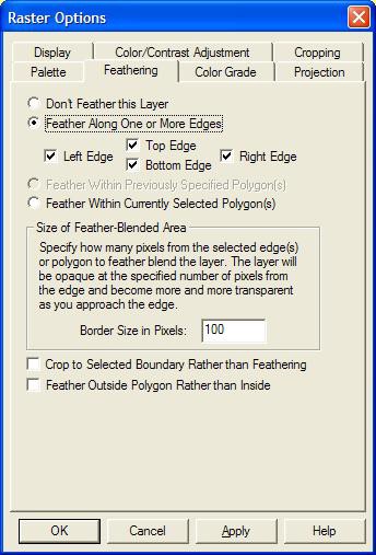
The
screenshot below displays the results of feather-blending a very high
resolution data set (0.15 meters per pixel) with a lower resolution (3.5 meters
per pixel) dataset to remove the edge. Note that the higher resolution image
has been purposely tinted violet to make the effect more obvious.

Color Grade Tab
The
Color Grade tab (pictured below) allows you to apply complex color correction
to a loaded raster file. You can setup the input range for each color channel
and what output range to map it to, as well as specify a saturation value.

Elevation Data Options
Selecting the Options...
button while only gridded elevation overlays are selected displays the
Elevation Options dialog. The Elevation Options dialog consists of two tabs,
one for controlling the display of the overlay(s) and the other for modifying
the elevation values within the overlay(s).
The Display tab (pictured below)
contains controls allowing you to control the color intensity
(brightness/darkness), color
transparency, blending, anti-aliasing, and color shading of the selected
layers.

The
Color Intensity setting controls whether
displayed pixels are lightened or darkened before being displayed. It may be
useful to lighten or darken raster overlays in order to see overlaying vector
data clearly.
The
Translucency setting controls to what
degree you can see through the overlay to overlays underneat the overlay. The
default setting of Opaque means that you cannot see through the overlay at all.
Settings closer to Transparent make the overlay increasingly more see-through,
allowing you to blend overlapping data.
The
Blend Mode setting controls how an
overlay is blended with underlying overlays, in addition to the Translucency setting. These settings
allow Photoshop-style filters to be applied to overlays, resulting in often
stunning results. What you get from a particular set of overlays from a
particular blend mode setting can often be hard to predict, so rather than try
to understand what is technically happening for each blend mode it's best to
just experiment with different ones until you find one that you like. The Hard
Light setting seems to work well with satellite imagery overlaid on DEMs, but
the others can be quite useful as well.
The
Transparent option allows a
particular color to be displayed transparently, making it possible to see
through a layer to the layers underneath. For example, when viewing a DRG on
top of a DOQ, making the
white in the DRG transparent makes it possible to see much
of the DOQ underneath. Pressing the Set
Transparent Color... button allows the user to select the color to treat as
transparent in the selected overlay.
The
Resampling option allows you to
control how the elevation value for each displayed/export location is
determined based on the values in the file. The following resampling methods
are supported:
• Nearest Neighbor - simply uses the value of
the sample that a location is in. When resampling or
reprojected an image this can result
in a stair-step effect, but will maintain exactly the original
elevation values of the source file.
• Bilinear Interpolation - determines the value of a
new sample based on a weighted average of the 4
samples in the nearest 2 x 2
neighborhood of the sample in the original image. The averaging has an
anti-aliasing effect and therefore produces relatively
smooth edges with hardly any jaggies.
• Bicubic Interpolation - a more sophisticated
method that produces smoother edges than bilinear
interpolation. Here, a new pixel is
a bicubic function using 16 samples in the nearest 4 x 4
neighborhood of the sample in the original image.
• Box Average (3x3, 4x4, 5x5, and 7x7) - the box
average methods simply find the average values of the
nearest 9 (for 3x3), 16 (for 4x4),
25 (for 5x5), or 49 (for 7x7) samples and use that as the value of the
sample location. These methods are very good for resampling
data at lower resolutions. The lower the resolution of your export is as
compared to the original, the larger "box" size you should use.
The
Shader option allows you to choose
which elevation shader is to be used for coloring the cell values within this
layer. By default, all gridded layers will share the elevation shader selected
on the toolbar, but there may be certain situations where you want to color one
layer differently than the others and exclude it
from the loaded elevation range. One common example is a
gridded layer that actually has non-elevation data.
The
Alter Elevation Values tab (pictured below) allows you to modify how elevation
values from the selected layer(s) are interpreted, providing you a means to
offset all of the elevations in the layer(s) by a given value and to restrict
the range of elevation values that are treated as valid.

Show/Hide Overlay(s)
Toggles
whether the currently selected overlays are visible. You can also use the
checkboxes next to each layer to control the visible state of the overlays.
Close Overlay(s)
Closes all the currently selected overlays.
3D View Menu Command
The 3D View command in Global
Mapper allows registered users to view gridded elevation data and any overlying
raster or vector data in a true perspective 3D manner. In addition, any vector
data with associated elevation values can also be displayed in true 3D.
VIDEO TUTORIAL ALERT!
• Video
Tutorial - Viewing 3D Vector Data
• Video
Tutorial - Creating a Custom 3D Map
When
selected, the 3D View command displays a window containing a 3D view of
the data in the current Global Mapper view.
Any imagery or vector data being drawn on top of the elevation grid(s) in the
main Global Mapper view will
automatically be draped on top of the elevation data in the 3D View window. If
so configured, any 3D vector data will be displayed in space as well.
The
image below depicts a sample of the 3D View window displayed using 250K USGS
DEM data for Salt Lake City, UT overlaid with DOQ satellite imagery from the
TerraServer import command under the File menu.

The image below depicts a sample of the 3D View window
displaying terrain data with 3D building areas for
Kuala Lumpur, Malaysia.
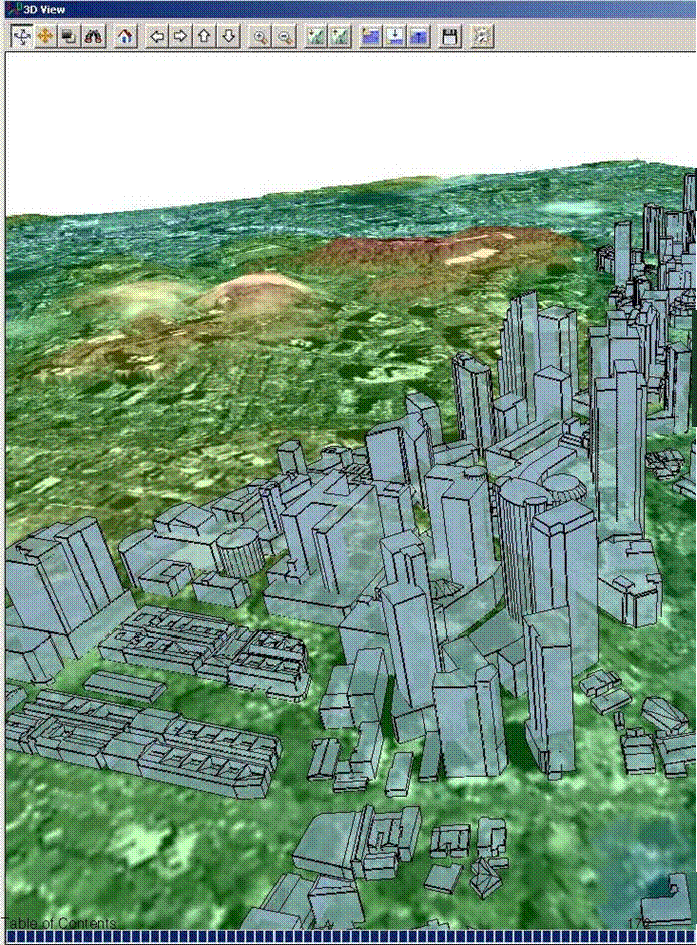
The 3D View window contains a toolbar with command buttons
allowing you to modify the default view.
You
can use the mouse to rotate the view around as well as zoom in. The arrow keys
on the toolbar allow you to pan the data visible in the 3D view in any
direction. The zoom in and out buttons allow you to zoom in or out on the
center of the 3D view. Additional buttons are also available for modifying the
vertical
exaggeration, displaying water, and saving the 3D view
contents to a Windows BMP, TIFF, PNG, or JPG file.
You
can also use the arrow keys and numeric keypad to pan and zoom the 3D
image without using the mouse. The following keys are recognized:
• Arrow
Keys: - pan 3D view left, right, forward, and back or move in
Walk Mode (hold shift for
larger
move).
• Page
Up/Down: - zoom in and out (hold shift for larger move)
• Numbers 8
and 2: - control tilt forward and back
• Numbers 4
and 6: - control rotation right and left
• Numbers 7
and 9: - move up
• Numbers 1 and
3: - move down
• Number 5
and letter H: - return to default view
• W: - show
wireframe
• A: - draw axes
If
you press the Change Display Properties button
on the 3D toolbar the 3D View Properties dialog
is displayed allowing you to configure the 3D view settings, including the
vertical exaggeration, the water display, background color, 3D vector display,
as well as the terrain and draped image resolution.
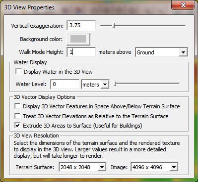
The
terrain and image size settings on the 3D View Properties dialog controls how
detailed the terrain surface and draped image surface in the 3D view will be.
Larger values will result in more detail, but will also take more time to draw.
Also some video cards can't handle the larger sizes, resulting in crashes in
the 3D view. If
this
happens and you can't get back into the 3D view options to change this, you
need to run 'regedit' and delete the 'HKEY_CURRENT_USER\Software\Global
Mapper\3DView_TextureSize' and
'3DView_TerrainSize' keys, then re-open the 3D viewer.
The
contents of the 3D View window will always reflect what is visible in the main Global Mapper view. This means that as
you pan and zoom around the main Global
Mapper view, the contents of the 3D View window will pan and zoom around as
well. The reverse is also true in that the pan and zoom buttons on the 3D View
window will cause the main Global Mapper view
to pan and zoom as well.
Another example of the 3D view is displayed below. This
time, it is several 24K USGS DLGs for Blue
Springs, MO overlaid on several 24K USGS DEMs for the same
area.

3D Vector Display - Advanced Discussion and Options
3D vector data is exaggerated along with the terrain so it
will align correctly. A bridge going over a gorge
with
heights of 100m and 110m on either end wouldn't match up with the terrain
heights of 100m and 110m if both weren't exaggerated. If relative elevations of
0m and 10m are used, those would end up as 0m and 30m
which would still allow the bridge to match up (NOTE: these
values assume a vertical exaggeration value of
3.0).
When
extruding to the surface, the default base of the extrusion is set just below
the minimum elevation, so your extruded areas should always extend through the
terrain surface.
You
can provide additional control over how 3D vector features are rendered by
provided attributes for those features. The supported attributes are as
follows:
• 3D_EX_HT -
the value of this attribute allows you to override the default extrusion height
and
extrude just that height in meters
• 3D_ZOFFSET
- the value of this attribute allows you to provide an additional offset (in
meters) when
rendering a 3D vector feature
Terrain Analysis Menu
The Terrain Analysis
Menu offers the following commands:
• Combine Terrain Layers
• Generate Contours Command
• Generate Watershed Command
• Find Ridge Lines Command
• Measure Volume Between Surfaces Command
Combine/Compare Terrain Layers Command
The
Combine/Compare Terrain Layers command allows the user to generate a new
gridded elevation (or other gridded value) layer by combining and/or comparing
the elevation values from two other loaded terrain layers.
When
selected, the command displays the Combine
Terrain Options dialog which allows the user to set up generation of the
new terrain layer. Once completed the new terrain layer is added to the Overlay
Control Center and displayed.
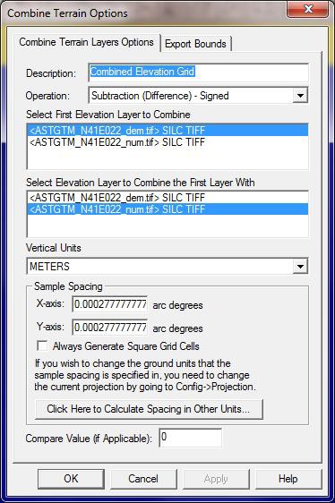
The
Combine Terrain Layers Options panel
(displayed above) allows the user to select the name to assign to the newly
generated layer, select the layers to combine to make the new layer, select the
operation to perform when combining the new layer, and select the vertical
units and sample spacing of the new layer. The available operations are
described below:
• Addition - values
from each layer are added to each other
• Subtraction
(Difference) - Signed - value in new layer is assigned to the difference
between the
value in the first layer and the
value in the second layer
• Subtraction
(Difference) - Unsigned - value in new layer is assigned to the magnitude
(absolute
value) of the difference between the
value in the first layer and the value in the second layer
• Average
Elevation - value in new layer is assigned to the average of the
value in the first layer and
the value in the second layer
• Minimum
Elevation - value in new layer is assigned to the smaller of the
value in the first layer and
the value in the second layer
• Maximum
Elevation - value in new layer is assigned to the larger of the
value in the first layer and
the value in the second layer
• Multiply
Values - value in new layer is assigned to the product of the
value in the first layer and the
value in the second layer
• Divide 1st
Value by 2nd - value in new layer is assigned to the value from the
first layer divided by
the value in the second layer. If
either value is missing or the second layer value is zero the new
sample is marked as invalid.
• Filter
(Keep First Value if Second Valid) - value in the new layer is
assigned to the value in the first
layer only if the value in the
second layer is vaild. Otherwise the value in the new layer is marked as
invalid (void). This is useful for applying a mask to a
terrain layer.
• Filter
(Keep First Value if Greater Than Second) - value in the new layer is
assigned to the value
in the first layer only if the first
layer value is greater than the second layer value. If either value is
invalid or the first value is less than the second value,
the value in the new layer is marked as invalid
(void).
• Filter
(Keep First Value if Less Than Second) - value in the new layer is
assigned to the value in
the first layer only if the first
layer value is less than the second layer value. If either value is invalid
or the first value is less than the second value, the value
in the new layer is marked as invalid (void).
• Filter
(Keep First if Second Greater Than Compare Value) - value in the new layer is
assigned to
the value in the first layer only if
the second layer value is valid and is greater than the specified
compare value. Otherwise the value is marked as invalid.
This is useful for keeping elevation values where something like a return count
from another layer is greater than some value. The Compare Value on the dialog
corresponds to the value to compare to.
• Filter
(Keep First if Second Less Than Compare Value) - value in the new layer is
assigned to the
value in the first layer only if the
second layer value is valid and is less than the specified compare
value. Otherwise the value is marked as invalid. This is
useful for keeping elevation values where something like an error value from
another layer is less than some value. The Compare Value on the dialog
corresponds to the value to compare to.
Note:
Only registered users of Global Mapper are able to combine terrain layers.
Generate Contours Command
The Generate Contours command allows
the user to generate equally spaced contour lines from any loaded
elevation grid data.
When
selected, the command displays the Contour
Generation Options dialog (pictured below) which allows the user to set up
the contour generation process.

The
Contour Options panel (displayed
above) allows the user to set the contour interval and units as well as the
grid spacing to use when generating the contours. You can also restrict the
elevation range within which contour lines are generated (by default all loaded
elevation values are considered). In addition, options are available to
generate isoheight area features in addition to contour lines as well as spot
elevations at the highest and lowest points in the area over which the contours
are generated. The smoothing option controls whether or not extra vertices are
added along generated line and area features to improve their appearance. If
you need to generate a huge amount of contour lines over a large area, the
option to export the contours directly to a package file can be used in
addition to the Gridding tab options to export those contours directly to
package files to get around memory limitations. Note that the contour lines
will be generated so that the
higher elevations are to the left of the contour line.
The
ADVANCED: Create Contours Where Elevations Pass Down to Contour Value Rather
Than as They Go Down From One option is an advanced option allowing you to
change how the contouring works in flat areas. If this option is checked, you
will get contours generated where the terrain surface arrives at a contour
height from higher terrain rather than where it departs a contour height for
lower terrain. So if you have a flat plain exactly at a contour height you will
get the contour at the base of the hill where it starts up rather than at the
top where it starts down. This is most useful when you have water (like the
ocean) and want to get a shoreline contour generated where the terrain leaves
the flat surface of the water.
The
Simplification panel (displayed
below) allows the user to set up the threshold at which points that don't
contribute much to the shape of the generated contour are removed in order to
generate lines with less vertices. The Gridding
panel allows you to break up your contour generation into smaller pieces
which can sometimes help reduce memory requirements when generating a very
large amount of contour lines. The Export
Bounds panel allows the user to set up the portion of the loaded elevation
grid data they wish to consider when generating the contours.

Generate Watershed Command
The
Generate Watershed command allows the user to perform a watershed analysis on
loaded terrain data to find stream paths as well as delineate the watershed
areas that drain into a given stream section. The
watershed calculation uses theeight-direction pour point algorithm (D-8) to calculate
the flow direction
at
each location, along with a bottom-up approach
for determining flow direction through
flat areas and acustom algorithm for automatically fllling
depressions in the terrain data.
When selected, the command displays the Watershed
Generation Options dialog (pictured below) which allows the user to set up the watershed generation process.


 Watershed Generation Options --
Watershed Options 1Watershed Bounds
1
Description ll•li!Hinfi11 1:115 •lil

 Resolution
The resolution affects
fidelity wdh which the watershed is generated.larger numbers result
in a less detailed watershed. but it will
generate more quickly. Typically you11 just want to accept the defauks.
 X-a:xis: 130 meters
 y-a:xis: 130 meters
K you wish
to change the ground units
that the resoh.!ltion is specified in, you need to change the current projection by going to Config>· Projection.
 Stream lhreshold
Specify how much ground
area or how
many cells
the flow
must accumulate from for a cell to be considered part of a stream. larger values resuk
in onty more major waterflows
being classaîed as streams.
r. Stream Cell Count 12500
 r Stream Drainage kea jo 1Square Meters
il
r Stream Drainage kea jo 1Square Meters
il
 r Discard Stream Starts Less than jso meters in Length
 Depression Rll
Depth
Depression Rll
Depth
Specify the maximum depth of depression inthe terrain data that will be filled
to facilîtate creating the flow network.
Reduce this fo.rfaster resu s.
1115 jmeters il
r Save DEM to GlobalMapper Gnd Rei Alter Rlling Depressions
P Keep Ocean Bevations .e.0meters)at Zero
 Operations at Selected Locations (Select wdh Digdizer Too)l
r Trace Aow from Selected Une(s}
r Trace Aowfrom Selected Point(s)\Water Drop Analysis)
r Create Watershed P<eas Showing Drainage
to Selected Une(s) r Create Watershed P<eas Showing Drainage to Selected Point(s) ADVANCED:Row lhreshold in Sampel
Resolution: j1
r
Create Watershed P<eas Showing
Drainage to Streams
P lnterpolate to Rll Small Gaps in Data
P Smooth Streams to lmprove Appearance
 r ADVANCED: Show
Row Accumulation as Gnd
r ADVANCED: Show
Row Accumulation as Gnd
1 OK 1
Cancel
1
Apply
 1
1
Help
1
The
Resolution section controls the resolution at which the loaded terrain data is
sampled to perform the watershed analysis. The default values should capture
the full resolution of the loaded terrain data. Larger values (i.e. lower
resolution) will cause the calculation to be quicker, but less detailed.
The
Stream Threshold section controls how much water must flow to a particular cell
before it is considered part of a "stream". Larger values will result
in only more water flow areas being delineated, while smaller values will cause
more minor water flows to be marked as streams. Each stream segment (i.e. the
portion between and inflow and outflow point) can optionally have the area that
drains directly to that stream segment marked with a watershed area. Check the
Create Watershed Areas Showing Drainage to Streams option to enable creating
watershed areas. If you would like to discard any short stream segments that
don't have any other streams flowing into them (i.e. short little stub streams
feeding into a main trunk), check the option to Discard Stream Starts Less than
Some Length. This will remove any short little stream stubs that are below
the specified distance threshold (in meters).
Many
terrain data sets will contain depressions in the data where flow would
terminate unless allowed to fill the depression and spill into the surrounding
terrain. The Depression Fill Depth section controls how deep of a depression
will be filled before it is considered a basin and flow is allowed to terminate
there. The depression fill depth value will automatically be filled in with
some guess at a good value based on the range of loaded elevation values, but
you might want to modify this, especially if you have relatively flat terrain
with a lot of depressions. Note that it can take a while to fill particularly
deep depressions. When trying to determine a a good value to use for the
depression fill depth you should think about how high of an embankment or 'dam'
that
you might encounter that you want to allow water to fill up to the top of and
pour over, or also how deep of a small pond or puddle to fill and allow
spilling out of. You can also check the option to Save DEM to Global Mapper Grid File After Filling Depressions to
save the depression-filled terrain to a GMG file so you can load that for
future watershed operations to avoid having to fill depressions again.
The
Operations at Selected Locations section
allows you to perform additional flow and drainage network delineation based on
line and point features selected in the Digitizer Tool. The Create Watershed Areas Showing Drainage to
Selected Line(s) option will calculate a drainage (watershed) area for each
selected line feature showing which portion of the loaded terrain drains to the
immediate vicinity (within the specified flow threshold) of the selected line.
This is useful to see what drains to something like a road feature. The Create Watershed Areas Showing Drainage to
Selected Point(s) option will calculate a drainage (watershed) area for
each selected point feature showing which portion of the loaded terrain drains
to the immediate vicinity (i.e. within the specified flow threshold of the
point location) of the selected point. The Trace
Flow from Selected Point(s) (Water Drop Analysis) option will cause a
separate arrowed line to be generated starting at each selected point feature
showing where a drop of water placed at that point location will flow to. The Trace
Flow from Selected Line(s) option will cause an area feature to be generated showing
all areas that a particular line feature will drain to. This is useful for
determining something like where a leak from a pipeline might
leak to.
The
screenshot below shows a watershed created from a collection of USGS DEMs. In
it you can clearly see the stream network as well as the drainage areas for
each stream segment.

@ Global Mapper v12.00 - REGISTEREO
.Eile ,Edit Vi· !ools earch §.PS J::!elp
<NO LABEL> Stream - (Height = 261.585 meters - <blue_springs_4_quads.dem> BLUE SPRINGS, MO)
 Find Ridge Lines Command
The
Fmd Ridge Lines command
allows the user to analyze the loaded terrain
data to find signiflcant ridge
!ines.The ridge linecalculation is
based heavily on the watershed generation algorithm, so see that for details on how it works.The main difference is that the ridge line operation simply inverts the terrain and where streams of water wouid forrn are now the ridge !ines in the inverted
terrain.
When
selected, the command displays the Ridge
Line Options Options dialog (pictured below) which allows the user to set
up the ridge line determination process.

Measure Volume Between Surfaces Command
The
Measure Volume Between Surfaces command allows the user to calculate the volume
between 2 terrain surfaces. When selected, the command displays a dialog
allowing you to select the 2 layers to calculate the volume between as well as
the region within which to do the volume calculation.
Tools Menu
The Tools Menu offers
the following commands:
• Zoom - Allows the user
to zoom in on a specific point in the display.
• Pan (Grab-and-Drag) - Drag the view to a new location.
• Measure - Measures length as well as an enclosed area.
• Feature Info - Chooses an object to display its attributes.
• Path Profile/LOS - Generate 3D path profile and perform line of
sight (LOS) calculations
• View Shed Analysis - Perform view shed analysis using loaded
elevation grid data
• Digitizer - Modify existing vector features and create
new ones.
• Image Swipe - Swipe away a raster layer to see what is
underneath
• Coordinate Convertor - Easy reprojection/conversion of coordinates
• Control Center - Central control for all loaded overlays.
• Configure - General Global Mapper setup.
• Map Layout - Setup Map Layout Display (scale bar,
margins, north arrow, etc.)
Zoom Tool 
The Zoom command selects
the zoom tool as the current tool.
To
zoom in on a specific point, choose the [Zoom tool] from the toolbar or,
[Tool/Zoom] from menu bar. A magnifying glass icon should appear on the screen.
To zoom in, left click without dragging the mouse. The view is centered on
where the mouse was clicked and will zoom in by a factor of two. To zoom out,
right click without dragging the mouse. The view will zoom out by a factor of
two, centered on where the mouse was clicked. You can also hold down the Ctrl key
while right clicking to restore the view to the last zoomed view.
Alternately,
one can zoom in to a user-defined rectangle by left clicking and then draging a
box while holding down the left mouse button.
If your mouse has a middle button, you can hold it down and
drag the map similar to the behavior of the Pan
(Grab-and-Drag) tool.
Pan (Grab-and-Drag) Tool

The Pan (Grab-and-Drag) command selects the Pan tool as the
current tool.
To
change the center point of the image without changing the magnification,
depress the left mouse button, drag the view to the desired location, then
release the left mouse button to redraw the view at the new location.
If you just want to recenter on a new location without
dragging, just click the left mouse button at the new desired location and the
view will be recentered on that location (this provides the functionality of
the old Recenter Tool).
Measure Tool 
The Measure command selects the measure tool as the current
tool.
To find the distance between along a path on the display or
the enclosed area of a set of points, choose the
[Measure Tool] icon from the toolbar or select
[Tools/Measure] from the menu bar.
1. Left click on the point to begin the measurement. Move
the mouse, which will draw a line, to the point where the measurement should
stop.
2. Repeat step 1 until you have defined the entire path or
area that you wish to measure.
3. Right click the right mouse
button and select "Stop Measuring" from the list using a left click.
Notice that "Stop Measuring" and "Close polygon" choices
are now grayed out. The measurement(s) will be displayed on the left side of
the status bar below.
4. In order to change measurements right click and choose a
new unit using a left click. You may continue to change the measurement display
by selecting different units. The distance will be displayed in kilometers,
meters, miles or feet for a line, and in square feet, square meters, square
miles, acres, or hectares for areas.
Note
that if you place a point along your measurement that you do not want you can
press Ctrl+Z to remove the last placed point in the measurement.
You
can also save a measurement to a separate feature by right clicking and
selecting "Save Measurement" from the list that pops up. You can then
export these measurements to new vector files, such as Shapefiles or DXF, or
modify them with the Digitizer Tool. There
is also an option to copy the measurement text to the clipboard when you
right-click.

If
you have gridded elevation data loaded under the measurement, you can also
calculate the Cut-and-Fill volume
either within the measurement area or within some distance of the measurement
line. To do this, simply right click then select the "Measure Volume
(Cut-and-Fill)" option that appears. Selecting this option will display
the Setup Volume Calculation Parameters dialog
(pictured below), which allows you to set up the volume measurement.

On
the Setup Volume Calculate Parameters you
can select whether to measure cut-and-fill volumes within some specified
distance of the selected line or within the specified area. If you are
measuring along a line, you can specify the cut heights to use at each vertex
individually or use the same cut (base) height for each vertex relative either
to the ground at each vertex or relative to sea level. Whichever option you
choose, the heights will be interpolated between line vertices to get a
smoothly varying cut height. If measuring within an area, there is also an
option to perform multiple cut-and-fill calculations between a range of cut
(base) height
values.
If you choose this option the results will be displayed in a table at the end
of the operation so you can see the results of each calculation.
Once you have your volume calculation setup and you press ok
to calculate it, the volume of earth that would be needed to fill any space
below the cut surface (fill volume) is reported along with the volume of earth
that is above the cut surface (cut volume). After viewing the reported volumes,
you have the option to save a new feature with the measurement values.
If
measuring the cut-and-fill volumes within an area feature, you can also check
the Find Area Cut Height Where Cut and
Fill Volumes are Equal to find the approximate cut height where the same
amount of dirt would have to be cut out as filled. This is useful for selecting
a cut height at which no dirt needs to be hauled off or brought in. The optimal
cut height will be reported as the break-even height with the other measurement
results.
On
the right-click menu in the Measure Tool are options to control how distances
are measured and the paths are drawn. The following options are available:
• Great
Circle - Any measured distances will use the great circle
distance, which is the shortest path
along
the surface of the earth's ellipsoid between the two points. Any drawn paths
will be along the
great circle path. Typically you won't notice a difference
for short distances, but will for longer ones.
• Grid
Distance - Any measured distances will use the distance as
calculated in the Cartesion XY
coordinate system of the current projected system. Any drawn
paths will be straight lines between the start and end point. This can result
in inaccurate distances for long measurements or when working in projection
systems with high levels of distortion.
• Rhumb Line
- Any measured distances will be drawn along the rhumb
line if possible, which is a line
of constant bearing between the
start and end point. Rhumb lines are often used in navigation so that a
constant bearing can be maintained. A rhumb line will be a
straight line in the Mercator projection. Any drawn paths will also be along
the shortest rhumb line path between the start and end point.
On
the right-click menu in the Measure Tool are options to control how bearings
are repoted. The following options are available:
• True North
- Any measured bearings will be reported relative to True
North. This means that a
bearing of 0 will point directly at
the North Pole and bearings of 180 will point directly at the South
Pole.
• Magnetic
North - Any measured bearings will be reported relative to
Magnetic North. This means
that a bearing of 0 will point
directly at the magnetic North Pole rather than the geographic North
Pole. All other bearings are relative to that, so a bearing
of 180 is exactly away from the magnetic North Pole. The magentic Nort Pole
slowly meanders around, but is not coincident with the geographic North Pole.
• Grid North
- Any measured bearings will be reported relative to Grid
North. This means that a
bearing of 0 will point directly up
on the Y axis of your current display projection (to the top of the
screen assuming you don't have any rotation enabled), 90
will be directly to the right along the X axis, etc. If your projection is one
that is orthogonal to the lat/lon grid, like Geographic or Mercator, the
cardinal directions (0, 90, 180, and 270) will be the same, but in between
could vary due to scale differences.
Feature Info Tool 
The
Feature Info command selects the Feature Information tool as the current tool.
This tool allows you to select vector features (areas, lines, and points) by
clicking on or near them. Once selected, a dialog displaying information about
the selected item appears.
To
pick objects, select the [Feature Info] icon from the Toolbar or select
[Tools/Feature Info] from the menu bar. Press and release the left mouse button
near the objects(s) to be picked. Holding down the 'P' key when left clicking
causes only area features at the clicked location to be considered. If
left-clicking on a picture point with an associated image, by default just the
image will be displayed, but holding the Ctrl key when clicking will cause the
normal feature info dialog to be displayed. When an object is picked, it will
be
highlighted
and a feature info dialog (picture below) will be displayed. Right clicking the
mouse button cycles through each of the elements located near the selection
point, displaying the information in the dialog box.

As
you can see, you can view a lot of information about a selected object in the
Feature Info dialog. The object's name, description, geometry information
including length and enclosed area (when applicable), attribute value list, and
map name, are all displayed. Buttons are also available allowing you to edit
the selected feature's information and drawing style, marking the selected
feature as deleted, as well as to copy all of the feature information (as text)
and the feature itself to the Windows clipboard for pasting elsewhere, such as
in a text editor or as a new feature in a running session of Global Mapper.
In
addition, you can right click on any attribute value to see additional options
specific to the selected attribute/value pair. You can copy the selected pair
to the Windows clipboard, treat the value as a web URL and open that location
in a web browser, or treat the value as a filename (either absolute or relative
to the path of the source file from which the feature was read) and load that
file either into Global Mapper or with the program associated with that file
type in Windows. You can also choose to zoom the main map view to the extents
of the selected feature.
If
the selected feature has an attribute named IMAGE_LINK and the value of that
attribute refers to a local image file, Global Mapper will automatically open
that image in the associated application on your system, unless the Ctrl button
was held down when you selected the feature. Likewise if you have an attribute
named GM_LINK and the value of that attribute refers to a local file, Global
Mapper will try and open that file in the current instance of Global Mapper as
a new layer, unless the layer is already open or the Ctrl key was held down.
Clicking
the Vertices button for line or area
features displays the Feature Vertex List dialog (pictured below), which allows
you to view, edit, and remove the individual vertex coordinates, including Z
and timestamp values (if present) for the selected feature. The X and Y coordinates
are listed in the native projection of the layer, and the Z coordinates will
have the elevation units defined for the layer on the Projection tab of the
Options dialog for the layer. You can also easily add per-vertex elevation
values to features that do not
already
have them by pressing the Add Elevs button
on the Feature Vertex List dialog. If timestamp values are present (like for a
GPS tracklog), speed and bearing columns will also be displayed for each leg of
the feature. You can also right-click on the vertex list for a feature with
per-vertex elevations and choose the option to evenly spread the elevations to
achieve a constant slope between the first and last elevation on the feature
and
also
to replace any zero elevation values by interpolating between non-zero values.
You can also add and edit per-vertex timestamps by right-clicking on the vertex
list and selecting the appropriate option.

Path Profile/LOS Tool 
The
PathProfile/LOS command selects the 3D path profile/LOS (line of sight) tool as
the current tool. This tool allows you to get a vertical profile along a
user-specified path using loaded elevation datasets. In addition, registered
users can perform line of sight calculations along the defined path.
To
define the path along which to generate the 3D path profile, first select the
path profile tool as your current tool. Press and release the left mouse button
at the position where you wish to start the path. Move the mouse to the next
position that you want to include in the path profile, then press the left
mouse button again. Right click on the last location in the path profile to
complete selecting points and display the Path
Profile/Line of Sight dialog (pictured below). The Path Profile/Line of Sight dialog will appear displaying the 3D
path profile of the selected path. Any points along the path that did not have
elevation data underneath will be treated as
an elevation of zero.
You can also generate 3D
path profiles for existing line features by selecting the line feature in
the Digitizer
Tool,
right clicking, then selecting the Generate Path Profile From Line option on
the menu that is displayed.

The
Path Profile/Line of Sight dialog
displays the 3D path profile and provides several options related to the
profile. A vertical scale is displayed on the left hand side of the profile
window. The start and end coordinates of the path are displayed at the top of
the profile window. If more than two points are in the path, the intermediate
points will be marked in the profile window with a yellow dot. These
intermediate points can be toggled on and off using an option available by
right clicking on the path profile window. Also note that this dialog is
resizable. If you have water display enabled on the Vertical Options tab of the
Configuration dialog and there would be water along the path, that will be
displayed as well.
Moving
your cursor over the profile window displays information about the current
cursor location along the profile, including the position and profile elevation
at the cursor location. You can get information about a portion of the profile
(a sub-path) by left clicking to start a sub-path definition, then
left-clicking again at the end of your desired sub-path. Details about the
sub-path, like length, elevation change, and slope, will then be displayed on
the bottom of the profile window.
Right
clicking on the profile window brings up an options menu allowing the user to
change the start and end positions, select the units (meters or feet) to
display the elevations in, configure display of the path profile, and display a
dialog containing details about the path. These options are also available
under the Options menu on the dialog.
The
File menu contains options allowing
you to save the path profile/line of sight data to a file. The individual
options are described below.
The Save To Bitmap... option
allows registered users to save the contents of the path profile window to a
Windows bitmap (BMP) file for use in other applications.
The
Save to BMP and Display on Main Map View option
allows registered users to save the contents of the path profile window to a
Window bitmap (BMP) file and then display that BMP at a fixed location on the
main map view. This is the equivalent of using the Save to Bitmap menu command, then closing the dialog and using the File->Open Data File at Fixed Screen
Location menu command in the main map view.
The
Save CSV File (with XYZ and Distance
Values... option allows registered users to save all of the coordinates and
distances to that location along the path profile to a CSV text file. Each line
in the text file will be formatted as follow:
x-coordinate,y-coordinate,elevation,distance-from-start
The
Save Distance/Elevation... option
allows registered users to save all of the distances and elevations along the
path profile to a text file. Each line in the text file will be formatted as
follow:
distance-from-start,elevation
The
Save To XYZ... option allows
registered users to save all of the positions and elevations along the path
profile to a text file. Each line in the text file will be formatted as follow:
x-coordinate,y-coordinate,elevation
The
Save LOS to KML... option allows
registered users to save a 3D line of sight and, if selected, the Fresnel zone
boundary lines, to a KML file for display in Google Earth.
Pressing
the Line of Sight... button brings up
the Setup Line of Sight/Earth Curvature dialog
(pictured below), which allows the user to configure a line of sight
calculation along the selected path. You can only perform a line of sight
analysis if exactly two points are in the path profile (e.g. line of sight
analysis cannot be performed on multi-segment paths).
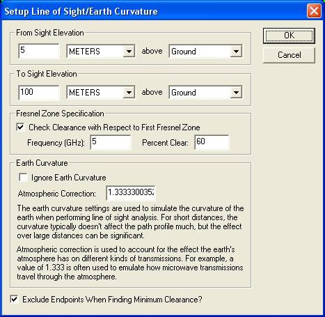
The
From Sight Elevation section allows
the user to select the height at the start position (left side of graph) to use
in the line of sight calculations. This height can be specified in either feet
or meters above the ground or above sea level. The To Sight Elevation section provides the same functionality for the
end position (right side of graph).
The
Fresnel Zone Specification section
allows you to have the line of sight analysis also check that a certain portion
(the Percent Clear value) of the
first Fresnel zone for a transmission of a particular frequency is clear. The
typical standard is that good visibility requires that at least 60% (the
default) of the first Fresnel zone for the specified frequency be clear of
obstructions. If Fresnel zone clearance is being selected the specified
percentage of the first Fresnel zone will be drawn on the line of sight
analysis dialog as a dotted line underneath the straight sight line.
The
Earth Curvature section allows the
user to specify whether they want to take the curvature of the earth into
account while performing the line of sight calculation. In addition, when earth
curvature is being used, they can specify an atmospheric correction value to be
used. The atmospheric correction value is useful when determining the line of
sight for transmitting waves whose path is affected by the atmosphere. For
example, when modeling microwave transmissions a value of 1.333 is typically
used to emulate how microwaves are refracted by the atmosphere.
Selecting
the Exclude Endpoints when Finding
Minimum Clearance options causes the first and last 5% of the elevations
along the profile to be ignored when finding the minimum clearance point.
After
setting up the line of sight calculation in the dialog and pressing the OK button, the line of sight will be
displayed in the path profile window (pictured below). Along with the line
depicted the actual line of sight, the position and vertical separation of the
minimum clearance of the line of sight will be displayed with a
dashed red line in the path profile window.

Pressing
the Cut-and-Fill Volumes... button
brings up the Setup Volume Calculation
Parameters dialog, allowing the user to perform a cut-and-fill volume
analysis along the path using loaded terrain data. See the Measure Tool for more information on cut-and-fill volume setup.
Once
you have performed a cut-and-fill analsyis, the cut line will be displayed on
the path profile allowing easy visualization of the cut and fill areas along
the path, as evidenced by the picture below.
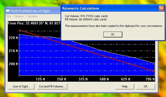
 View Shed Tool
The
View Shed command selects the view shed analysis tool as the current tool. This
tool allows registered users to perform a view shed analysis using loaded elevation
grid data with a user-specified transmitter location, height, and radius. All
areas within the selected radius that have a clear line of sight to the
transmitter are colored with a user-specified color.
To
perform a view shed analysis, first select the view shed tool as your current
tool. Press and release the left mouse button at the position where you wish to
place the transmitter. At this point, the View
Shed Setup dialog (pictured below) will appear, allowing you to setup the
view shed calculation.
You can also calculate views
sheds at multiple point locations by selecting the point features at the
desired locations in the Digitizer Tool,
right clicking, then selecting the Calculate View Sheds at Selected Point(s)
option on the menu that is displayed.
If
you choose to perform view shed operations at selected point feature locations,
the view shed calculation values will be initialized from attributes of that
point feature. The values selected on the dialog will be used, except when one
of the following attributes is present with a value to override what was
selected on the dialog (this allows you to batch calculate view sheds at
different locations with different parameters):
• OFFSETA -
height above ground in meters (or feet if 'ft' in value) for transmitter
(observation point)
• OFFSETA_MSL
(or OFFSETA_MS if coming from a Shapefile) - height above sea level in meters
(or feet if 'ft' in value) for
transmitter (observation point)
• OFFSETB -
height above ground in meters (or feet if 'ft' in value) for receiver
• OFFSETB_MSL
(or OFFSETB_MS if coming from a Shapefile) - height above sea level in meters
(or feet if 'ft' in value) for
receiver
• AZIMUTH1 -
start angle for view shed (0 is north, 90 is east, etc.)
• AZIMUTH2 -
send angle for view shed (0 is north, 90 is east, etc.)
• RADIUS2 -
outer radius in meters of view shed calculation
• RADIUS1 -
inner radius in meters of view shed calculation (default is 0, which does
entire radius)
• VERT1 -
The top of the vertical angle to limit the scan (receiver angle range top
value)
• VERT2 -
The bottom of the vertical angle to limit the scan (receiver angle range bottom
value)

The View Shed Setup dialog
provides options that allow the user to precisely setup the view shed analysis
that they wish to perform.
The Description provides
the user with a place to enter a name to identify this view shed analysis. This
name will be displayed in the Overlay Control Center and will also be the name
of the transmitter point created by the analysis for display on the map.
The Transmitter
Elevation section allows the user to specify the height of the transmitter
that the view shed analysis will be simulating.
The Receiver Elevation
section allows the user to specify the minimum height above the ground or
sea level from which the transmitter must be visible for the
point to be considered visible. Most of the time you'll want to specify an
elevation above ground, but specifying an elevation above sea level can be
useful for aviation purposes.
Optionally, you can also specify that the receiver elevation
should be calculated based on an elevation angle relative to the horizon from
the transmitter. This is useful if you have something like a radar
dish that points up at some angle and you want to see where
the signal can be seen.
Finally, you can also specify a transmission angle range for
a beam transmitted from the transmitter. Then the view shed will depict where
that beam would hit the terrain surface (or some user-specified distance above
the surface).
The Select Elevation
Layer(s) to Base Transmitter/Receiver Heights On button displays a dialog
allowing you to select which of the loaded elevation layers you want to base
ground-relative transmitter and receiver heights on. The default is to use all
loaded layers, but if you have a situation where you have a ground level data
set loaded and perhaps another set with heights of buildings, etc., you could
use this option to cause the transmitter and receiver heights to be based on
the ground elevation, whereas the actual visibility of each point will use the
topmost of any loaded layer.
The View Radius section
allows the user to specify how far in each direction from the transmitter to
check for visibility. Typically you'd want to set this to the effective range
of your transmitter. If you want to ignore areas close to the transmitter, you
can also specify a minimum view radius value.
Use the default of 0 to include everything from the transmitter out ot the
selected view radius.
The View Angle section
allows the user to limit the view shed to a particular subsection of the
complete radial area. The Start Angle specifies
the cartographic angle at which the radial subregion begins. This angle is a
cartographic angle, meaning that 0 degrees is north and angles increase
clockwise. The Swept Angle specifies
the number of degrees clockwise to include in the view shed. For example, if
the transmitter being analyzed sweeps an arc from due south to due west, a
start angle of 180 with a swept angle of 90 would be used. To perform a view
shed analysis over the entire area, keep the defaults of starting at 0 degrees
and sweeping through 360 degrees.
The Earth Curvature section
allows the user to specify whether they want to take the curvature of the earth
into account while performing the view shed analysis. In addition, when earth
curvature is being used, they can specify an atmospheric correction value to be
used. The atmospheric correction value
is
useful when determining the view shed for transmitting waves whose path is
affected by the atmosphere. For example, when modeling microwave transmissions
a value of 1.333 is typically used to emulate how microwaves are refracted by
the atmosphere.
The Sample Spacing section
allows the user to specify the spacing of elevation samples when calculating
the view shed. The sample spacing controls the interval at which elevation
samples are examined to determine visibility. Smaller values result in more
accurate, but more slowly generated, view sheds.
The Fresnel Zone
Specification section allows you to have the view shed analysis also check
that a certain portion (the Percent Clear
value) of the first Fresnel zone for a transmission of a particular
frequency is clear. The typical standard is that good visibility requires that
at least 60% (the default) of the first Fresnel zone for the specified
frequency be clear of obstructions. If you specify a maximum Fresnel zone
percentage clear other than 100%, only those locations where the minimum
percentage of the 1st Fresnel zone that is clear is between your specified
percentages will be marked
as visible.
The
Free Space Path Loss Calculation section
allows you to display the power at any given location taking free space path
loss into account. You can specify the total power from the rest of the link
budget (i.e. transmission power plus antenna gain minus any other power losses
excluding free space path loss) and the signal frequency. Then as you move the
cursor over the view shed you can see the remaining power at the location. In
addition the view shed will get more transparent as thed signal power becomes
less.
The
Obstructions from Vector Data section
allows the user to specify whether or not loaded vector data with elevation
values should be considered when performing the view shed analysis. This allows
the user to use things like buildings, fence lines, towers, etc. to block
portions of the view, creating a more realistic view shed. If the user elects
to use vector data, they can also specify whether the elevation values stored
with vector features are relative to the ground or relative to mean sea level.
Typically heights for vector features are specified relative to the ground. If
any area features are included and their heights are relative to the ground,
the obstruction heights within those areas will be increased by the specified
amount, but any receiver heights will still be based on the terrain. This makes
things like wooded areas very easy to model. The Obstruction Area Features Always Hidden option allows you to
specify that any locations within an obstruction area will be marked as hidden,
rather than only those that actually would be hidden.
If checked, the Display
Hidden Rather than Visible Areas option causes the generated view shed to
cover those areas that would NOT be visible, rather than those that would be
visible from the transmitter location.
If checked, the Generate
Area Features in Covered Areas option specifies that view shed coverage
area (polygon) featuers should be generated for those areas that are visible.
These generated area features then behave just like any other vector feature
and can be exported to vector formats, like Shapefiles, for use in other
software.
Pressing the Select
Transmitter Location... button displays a dialog that allows the user to
adjust the exact transmitter coordinates from the coordinates where they
clicked.
Pressing the Select
Display Color... button displays a dialog that allows the user to select
the color in which to display the visible areas on the map.
After setting up the view shed calculation in the dialog and
pressing the OK button, the view shed
analysis will be performed and when complete, the results will be displayed on
the main map display as a new overlay. All visible areas within the specified
radius will be displayed using the selected color. The overlay will default to
being 50% translucent, allowing you to see areas underneath the view shed. You
can modify the translucency of the overlay in the Overlay Control Center.
In addition, a small radio tower point will be created at
the selected transmitter location. When selected using the pick tool, this
point displays information about the view shed analysis as shown below.
If you would like to modify the settings used to calculate
the view shed and recalculate it using currently loaded data, you can right
click on the View Shed layer in the Overlay Control Center and select the
option to modify the view shed.

Image Swipe Tool
The Image Swipe command selects the image swipe tool. This
tool allows you to select a raster/image layer to swipe away by holding down
the left mouse button and dragging in some direction. This allows you to easily
compare overlapping layers in an interactive manner.
You will be prompted to select the raster/image layer to
swipe away when activating the tool. Once active, you can change the swipe
layer by right-clicking and choosing the appropriate option. To swipe, just
hold down the left mouse button and drag in the desired swipe direction. When
you release the mouse the swipe is reset and the entire image is displayed
again.
Coordinate Convertor Command
Selecting the Coordinate Convertor... menu item displays the
Coordinate Convertor dialog (picture
below). This dialog allows you to easily convert a coordinate in one
projection/datum/unit system to another. When a conversion is made the results
are automatically copied to the clipboard for easy pasting in another location
using Ctrl+V. There are also buttons to allow you to easily recenter the map on
the coordinates or to create a new point feature at the coordinates.
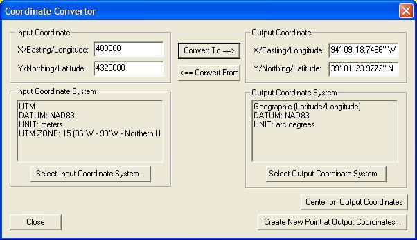
 Control Center Command
Selecting the Control Center... menu item or toolbar button
displays the Overlay Control Center dialog.
This dialog is the central control center for obtaining information and setting
options for all loaded overlays. See the Overlay
Control Center section for complete details.
Configure Command 
Selecting
the Configure... menu item or toolbar button displays the Configuration dialog. This dialog provides for general setup of
Global Mapper display options. See the Configuration
section for complete details.
Map Layout Command
Selecting the Map Layout... menu item or toolbar button
displays the Map Layout dialog
(pictured below). This dialog provides for setup of the map display, including
specifying the placement and display of the distance scale bar, elevation
legend, margins, map legend and north arrow. There are also options to save and
map layout to a file and restore it later. In addition, the current map layout
will be saved to any workspace files.

The Map Legend section
allows you to setup the display of a map legend on the display. You can setup
your map legend to use one of the following types:
♦ No Map Legend - no map legend is displayed
on the map.
♦ Display Legend Based on Loaded Vector Types - a map
legend is generated based on the list
of loaded vector types and their
drawing styles. There will be a separate entry on the legend
for each unique combination of type and style. You can
filter the list of type that are displayed on the map legend using the Filter
Types button.
♦ Display Legend Based on Color Palette - a map
legend is generated based on a color palette
(i.e. a list of colors and names.
You can setup the palette to use for generating the map legend
using the Setup Palette button. On that dialog you
can manually enter colors and their names, load a palette from a file, or
initialize a palette from the palette of a loaded file.
♦ Display Legend Based on Vector Types and Palette - this
option is a combination of the
previous two item. Both entries from
the loaded vector types/styles and from a customizable
color palette will be used.
 Digitizer Tool
The
Digitizer Tool allows you to modify existing vector features as well as to
create new ones. This tool encompasses a lot of functionality, from modifying
the shape and position of area, line, and point features, to editing the
attribution and drawing styles of individual vector features. The major
activities available with the Digitizer Tool are described below.
• Creating New Features
♦ Creating New Area Features
♦ Creating New Line Features
♦ Create New Line Features with Distance/Bearing/COGO Input
♦ Creating New Point Features
♦ Creating New Range Ring Features
♦ Create Buffer Areas a Fixed Distance Around Features
♦ Creating Shape (e.g. Circle, Rectangle, etc.) Features
♦ Create Strike-and-Dip (Geology-Related) Features
♦ Create Regular Grid of Area Features of User-Specified
Size/Orientation
♦ Create Points Spaced Along Area and Line Features
♦ Creating a Line by Connected Points
♦ Create Perpendicular Lines Spaced Along Area and Line
Features
♦ Creating a Point Offset from a Selected Point
• Editing Existing Features
♦ Selecting Features
♦ Selecting Vertices
♦ Editing Feature Attributes and Drawing Styles
♦ Deleting/Undeleting Features
♦ Moving Features
♦ Changing the Shape of Area and Line Features
♦ Rotating and Scaling Features
♦ Combining Area and Line Features
♦ Finding the Intersection of Multiple Area Features
♦ Cutting Areas From/Adding Islands to Area Features
♦ Splitting Areas into Two New Area Features
♦ Cropping Features to Selected Area Features
♦ Cropping/Splitting Line Features to Area Features
♦ Splitting Area Features Against Line Features
♦ Moving Selected Point Features to the Nearest Point on
Selected Line Features
• Copying Features (Cut/Copy/Paste)
• Snapping to Existing Features When Drawing
• Snapping Vertically/Horizontally When Drawing
• Un-doing Digitization Operations
• Additional Feature Operations
♦ Adding Elevation Values from Terrain to Features
♦ Generating a 3D Path Profile from a Line or Area Feature
♦ Calculating View Sheds at Multiple Point Locations
♦ Calculating Elevation Statistics for Selected Features
♦ Calculating Cut-and-Fill Volumes for Area and Line
Features
♦ (Global Energy Mapper only) - Insert a Pad Site Template
♦ (Global Energy Mapper only) - Creating a Flattened Site Plan
♦ Working with Feature Measurements (i.e. Length, Enclosed
Area)
♦ Automatically Inserting Vertices at Line Intersections
♦ Finding Non-Connected Line Endpoints (i.e. Connectivity
Checks)
♦ Finding Nearby Points
♦ Flattening Terrain Using Area Features
♦ Adding Address Information to Points from Nearby Road
Features
♦ Adding Coordinate Attributes to Point Features
♦ Adding Attributes to Features from Other Featuresmike1460
♦ Counting Features Contained within Area Features
♦ Converting Areas with Islands to Single Vertex List
♦ Connect Points to Selected Lines with Shortest Path Line
Creating New Features
At
any time that the Digitizer Tool is active, you have the option to create new
area, line, and point features simple by right clicking and selecting either
the Create
New Area Feature, Create New Line Feature (Vertex or Trace Mode), or Create New Point Feature options
on the popup menu (pictured below). Any new features created can be exported to
new vector files in any of the supported vector export format (DXF, Shapefile,
etc.).

Creating New Area Features
After
selecting the Create New Area Feature popup
menu option, you can proceed to draw a new area feature with the mouse. To draw
the feature, simple left click at each place that you'd like to drop a vertex.
To finish the area feature, right click at the desired location of the last
vertex to complete the area. You can cancel creation of the new area at any
time by pressing the Escape key. Note that while drawing the area you can use
the Snapping
feature to help align the area with existing features.
Once
you've completed drawing the area, the Modify
Feature Info dialog will appear allowing you to setup the label,
classification, drawing style, and attribution for the area. The perimeter and
enclosed area of the area feature will be added as default attributes. The
units for these measurements can be modified on the General tab of the Configuration
dialog. See Editing Feature Attributes and Drawing Styles for more details.
Once
you have completed have completed creating the area, the Digitizer Tool will
remain in the area creation mode, so you can simply start left-clicking to draw
another area, or right-click to choose a different mode.
You
can also create new area features from selected line features by selecting a
collection of lines, then right-clicking and selecting the Advanced Feature Creation Options->Create New Area Feature(s) from
Selected Line Feature(s) menu command. This will attempt to connect the
selected line features to build area features. All line features will be
connected as far as possible, then closed to create a new area feature. When
you select this option, the dialog shown below will appear allowing you to
setup the rules governing how areas will be formed. The rules have the
following meanings:
• Only
Connect Lines that Match the Attributes of the Line Being Connected To - If
checked, this
option indicates that line features
will only connect to other line features that have compatible labels,
descriptions, and attributes.
• Require
Connected Results to be Fully Closed Before Creating Area - If checked, this
option indicates
that only connected line paths that
fully close to form a complete area will be turned into areas. If not
checked, any path will be closed with a straight line
between the two endpoints once no more connections can be found.
• Create
Multiple Areas if All Lines Don't Connect - If checked, this option indicates
that if all of the
selected lines don't connect to form
a single path, then multiple area features will be generated, one
for each independent connected path.

Creating New Line Features
After
selecting the Create New Line Feature
(Vertex Mode) popup menu option, you can proceed to draw a new line feature
with the mouse. To draw the feature, simple left click at each place that you'd
like to drop a vertex. To finish the line feature, right click at the desired
location of the last vertex. You can cancel creation of the new line at any time
by pressing the Escape key. Note that while drawing the line in Vertex Mode you
can use the Snapping feature to help align the line with existing features.
You
can also choose to draw a line using the Create
New Line/Area Feature (Trace Mode) popup menu option. To draw the feature,
simple press the left button to start the line/area, then trace the path to
draw using your mouse while keeping the left button pressed. To finish the
feature, simply release the left button. You
can cancel creation of the new feature at any time by
pressing the Escape key or just releasing the left button then pressing Cancel
on the dialog that appears. If you are using a digitizing table just select
this mode, then press down the pen to start, trace the path, then release it to
end. If your drawn path is nearly closed, you will be asked whether to create a
closed area feature from the path or just keep it as a line feature.
Once you've completed drawing the line, the Modify Feature Info dialog will appear
allowing you to setup the label, classification, drawing style, and attribution
for the line. The length of the line feature will be added as a default
attribute. The units for the length measurement can be modified on the General tab of the
Configuration dialog. See Editing Feature Attributes and Drawing Styles for
more details.
Once
you have completed have completed creating the line, the Digitizer Tool will
remain in the line creation mode, so you can simply start left-clicking to draw
another line, or right-click to choose a different mode.
You can also create new line features from selected area
features by selecting one or more areas, then right-clicking and selecting the Advanced Feature Creation Options->Create
New Line Feature(s) from Selected Area Feature(s) menu command. This will
create a single closed line feature from each selected area feature.
Creating New Line Features with Distance/Bearing/COGO Input
After
selecting the Create New Line with
Dist/Bearing/COGO popup menu option, you can proceed to select the starting
location of the new line feature by left clicking at the desired start
location. Note that while selecting the start point for the line you can use
the Snapping
feature to help align the line with existing features.
After
selecting the starting location, the Distance/Bearing/COGO Input dialog
(pictured below) will display, allowing you to enter distance/bearing
information for additional points either as separate distance/bearing values,
as a COGO (Coordinate Geometry) coordinates (see below for explanation), or as
a quadrant/bearing/distance value. Once you have entered all of your points,
press Done to complete the process and create the new line feature.
You
can also check the option to Close Path
Using Compass Rule when Completing Feature. If this option is checked, all
of the points will be adjusted using the compass rule to ensure that the shape
is closed. The compass rule evenly distributes the shift required to close the
shape to all vertices and is commonly used by surveyors.

One Handed Entry of Values
You
can achieve very fast entry of large collections of distance/bearing of
quadrant/distance/bearing values by simply using the number pad and pressing
Enter after each value. This will take you to the next field and finally add
the point when you press Enter on the last field. This will also take you back
to the first field to allow continuously adding points with only one hand,
keeping your other hand free to mark your place on the list of values.
Notes on Bearings
When
entering data using the Specify Separate
Distance and Bearing Values option, the bearing values are degrees
clockwise from true north, so 0 degrees is north, 90 degrees is east, etc. For
the Specify Using
Quadrant/Bearing/Distance option, you specify a quadrant value of 1 to 4,
with 1 being the NE quadrant, 2 being the SE quadrant, 3 being the SW quadrant,
and 4 being the NW quadrant. The bearing values are then east of the NS line
for quadrants 1 and 2 and west of the NS line for quadrants 3 and 4.
It is also important to remember that any bearing are
specified relative to true north (unless you check the Use
Grid Bearings Rather Than Bearing
Relative to True North), so if your projection isn't
oriented so that straight up is true north (most projected systems, like UTM,
are not unless you are right at the projection
center) a line of bearing 0 won't be straight up, but will
be slightly skewed so that it points at the North Pole. A line of bearing 0
will be straight up in projections like Geographic or Mercator where true north
is always straight up.
If
you check the DMS (degree/minute/second)
Values Specified in Decimal Degrees option, you can enter your DM
(degree/minute) or DMS (degree/minute/second) values as decimal degrees. For
example with this option checked, a value of 40.3020 is interpreted as 40
degrees, 30 minutes, and 20 seconds. The basic format of degree fields when
this option is checked is DD.MMSS.
Example COGO Input
N 23:14:12 W 340
S 04:18:56 E 230
The
first character of a COGO input string must be either the character 'N' or 'S'
to indicate whether the bearing is relative to the north or south directions.
After another space, the angle begins. The angle can be in any angle
specification that Global Mapper supports, including degrees, degrees/minutes,
or degrees/minutes/seconds. A space follows the angle, and is then followed by
either the 'E' or 'W' characters. A space separates the bearing from the
distance (which should be in appropriate linear units).
For those unfamiliar with the notation for bearings: Picture
yourself in the center of a circle. The first hemispere notation tells you
whether you should face north or south. Then you read the angle and either turn
that many degrees to the east or west, depending on the second hemisphere
notation. Finally, you move distance units
in that direction to get to the next station.
Creating New Point Features
After
selecting the Create New Point Feature popup
menu option, you can proceed place the point feature by left clicking at the
desired location of the point. You can cancel creation of the new point at any
time by pressing the Escape key.
You can also use the Create
New Point Feature at Specified Position option to create a new point
feature at a manually specified location. When you select this option, a dialog
appears allowing you to enter the location for the new point feature in either
latitude/longitude coordinates or coordinates in the current view projection.
Once you've placed the point, the Modify Feature Info dialog will appear allowing you to setup the
label, classification, drawing style, and attribution for the new point
feature. See Editing Feature Attributes and Drawing
Styles for more details.
Once
you have completed have completed creating the point feature, the Digitizer
Tool will remain in the point creation mode, so you can simply left-click to
place another point, or right-click to choose a different mode.
You can also create new point features from the centroids of
selected area features or from the vertices of selected line and area features
by selecting one or more areas or lines, then right-clicking and selecting the
appropriate option under the Advanced
Feature Creation Options menu.
Creating New Range Ring Features
After
selecting the Create Range Ring(s) popup
menu option, you can proceed to place the center location of your range rings
by left clicking at the desired location. If you had point features selected
when you selected
this
option you can also choose to create the rings centered on the selected point
feature(s) rather than manually specifying a center location. You can cancel
creation of the range ring(s) at any time by pressing the Escape key or right
clicking. If you choose to create new range rings at selected point locations
and those points have a RING_RAD_M attribute, that attribute value will be
interpreted as the ring radius in meters and used rather than what is specified
in the dialog described below.
After
selecting the center of your range ring(s), the Select Range Ring Parameters dialog (pictured below) appears and
allows you to setup how many range rings you would like to create and how far
apart you would like to create them. You can choose to create rectangles with the
specified range as the radius rather than a ring if you would like. You can
also choose to create a "multi-ring". Checking this box will delay
the actual range ring creation until you have added additional range rings and
unchecked the box. Then all rings in the "multi-ring" will be
combined if possible to build nice looking combined range rings.
Once you have completed have completed creating the range
ring(s), the Digitizer Tool will remain in the range ring creation mode, so you
can simply left-click to create additional range rings centered on another
location, or right-click to choose a different mode.
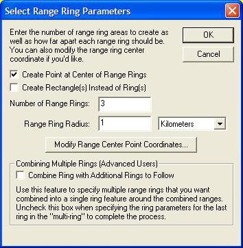
The range ring feature has numerous applications, including
search-and-rescue and aviation. Creating Buffer Areas Around Selected Features
After selecting the Create Buffer Areas Around Selected
Feature(s) option in the Advanced
Feature Creation
popup
menu, the Setup Buffer Areas dialog
(pictured below) appears and allows you to setup how many buffer areas that you
want to create around each selected feature and at what distance to space them.
For example, if you want to create buffers at distances of 100, 200, and 300
meters around each selected feature, you would specify that you want to create
3 buffer areas with a buffer distance of 100 meters. You can also select to get
the base buffer distance from an attribute of the selected features rather than
using a single fixed buffer radius for each feature. That attribute value can
also include unit text, like '500 m' or '300 ft' and that will automatically be
recognized and used. If you would like to combine all overlapping buffers into
larger combined areas, simply check the option to Combine Overlapping Buffer Areas. To create buffers some
distance inside a selected area feature rather than outside
of it, simply specify a negative buffer distance.
Once
you have completed have completed creating the buffer areas(s), the newly
created areas will automatically be selected so you can easily right-click to
edit them, display measurement information, etc.

Creating New Shape (e.g. Circle, Rectangle, etc.) Features
Under
the Create Area Shapes and Create Line Shapes right-click popup
menus you will find options to create Arc, Circular, Elliptical, Rectangular,
and Square area and line features. For all of these shape types (except the
rectangular/square option where you manually enter the coordinates), you click
and hold the left mouse button at the center of the feature, then drag it until
it is of the desired shape. For Circular/Elliptical features and Arcs, the
default shape follows a circle and holding down the SHIFT key will dragging
will result in an ellipse. For Rectangular/Square features, the default shape
is a rectangle and holding down the SHIFT key will force the dragged shape to
be square. If you hold down the 'T' key when left clicking to start the
shape,
the start point will be treated as the top left corner of the feature rather
than the center of the shape feature.
If
you choose the 3-point area or line rectangle creation options, you enter a
special mode for easily drawing rotated rectangles. Just left click to start
the rectangle, then left-click again at the end of the first side, then left
click again when the rectangle shape is what you want to create it.
Once
the shape is to your liking, release the left mouse button and the Modify Feature Info dialog will appear
allowing you to setup the label, classification, drawing style, and attribution
for the new feature. See Editing Feature
Attributes and Drawing Styles for more details.
Once you have completed have completed creating the shape,
the Digitizer Tool will remain in the selected shape creation mode, so you can
simply start drawing a new shape, or right-click to choose a different mode.
Create Strike-and-Dip (Geology-Related) Features
After
selecting the Create Strike-and-Dip Point
popup menu option, you can proceed to select the location of your new point
by left clicking at the desired location. If you drag the cursor in the
direction of the strike then
release
it, the point will be placed at the start of the mouse drag and the strike/dip
azimuth will automatically be initialized to the direction that you dragged.
You can cancel creation of the point(s) at any time by pressing the Escape key
or right clicking.
After
selecting the locationof your strike-and-dip point, the Enter Strike-and-Dip Parameters dialog (pictured below) appears and
allows you to setup your point. This includes selected the azimuth angle for
your strike, either relative to True North (the default) or to the top of the
map screen, the dip value for your point (which will be used as the display
label on the map), the symbol to use, an optional description, and which layer
in
the
Control Center to place the new point feature. There is also a Modify Location button which allows you
to fine-tune the location of the point by manually entering coordinates.
Once
you have completed have completed creating the strike-and-dip point, the
Digitizer Tool will remain in the strike-and-dip creation mode, so you can
simply left-click to create additional points centered on another location, or
right-click to choose a different mode. If you hold down the Ctrl key when
left-clicking to create additional points the new strike-and-dip point will
automatically be created at the clicked location using the same parameters as
the last strike-and-dip point that was created, allowing you to quickly place a
lot of points without going through the dialog each time.

Create Regular Grid of Area Features of User-Specified
Size/Orientation
After
selecting the Create Regular Grid of User
Specified Size/Orientation popup menu option, you can proceed to select the
anchor point (top left corner) of your grid by left clicking at the desired
location. You can cancel creation of the point(s) at any time by pressing the
Escape key or right clicking.
After
selecting the anchor point for your grid, the Grid Setup dialog (pictured below) appears and allows you to setup
the size, count, naming, and orientation of your grid cells. Pressing the Anchor Point button allows you to edit
the location of your anchor point. You can also choose to create lines rather
than areas and to
create
points at the grid edges if you want, which is useful for creating your own
labeled grid over the map for just a certain sub-area.

Create Points Spaced Along Area and Line Features
You
can create new point features evenly spaced along a selected area and line
features by right clicking and selecting the Advanced Feature Creation submenu
option Create Point Features Spaced Along
Selected Feature(s). This will present a dialog allowing you to specify the
spacing to use, then create new point features at the specified interval along
the line.
Create Line by Connecting Selected Point Features
You
can create a new line feature by connecting selected point features by right
clicking and selecting the Advanced Feature Creation submenu option Create Line from Selected Point Features.
This will find a path from the selected points (starting at the first selected
point and then adding the closest point to each end until all of the point are
connected), then create a line feature from that path.
Click Here for Video Tutoral
Create Perpendicular Lines Spaced Along Area and Line
Features
You
can create a new line features spaced along selected area/line features that
are perpendicular to those selected features at each point. To do so, first
select one or more area/line features, then right click and selecti the
Advanced Feature Creation submenu option Create
Perpendicular Lines Spaced Along Selected Line/Area Feature(s).... You will
be prompted to select the spacing between lines and also the total length of
each perpendicular line.
Creating a Point Offset from a Selected Point
You can create a new point feature offset a given
distance/bearing or X/Y offset from an existing point by selecting the start
point feature, then right clicking and selecting the Advanced Feature Creation
submenu option POINT AT OFFSET - Create
New Point/Text Feature At Specified Bearing/Distance.
Editing Existing Features
In addition to creating new vector features, the Digitizer
Tool is also very useful for editing existing vector features. This tool
provides the ability to move, delete, and reshape vector features, as well as
modify the label, classification, drawing style, and attribution of any vector
feature loading from any file format supported by Global Mapper. Note than any
edits made are NOT automatically saved back to the origin file, but they will
be saved in Global Mapper workspaces and into any exported vector files.
Selecting Features
Before
you can edit an existing feature or features, you first must select them. Once
a feature is selected, you can tell that it is selected because it will be
drawn with a different style. The different methods for actually selecting
features are described below.
One
way to select features is by simply by clicking the left mouse button near the
feature, or in the case of area features, within the feature. Using this
method, the closest point or line feature will be selected, or if no point or
line features are nearby and you clicked within an area feature, the area
feature will be selected.
To
select multiple features at a time, you can drag a selection box by holding
down the left mouse button to draw a box. Any features entirely within the box
drawn or features which are cut by the box will be selected. If you hold down
the 'I' key while dragging the box, only features and vertices that are
completely within the box will be selected. This is useful for things like
selecting a point feature that is on top of a line/area border.
You
can add to an existing selection by holding down the CTRL key while performing
a selection with any of the above described methods. You can deselect features
by holding down the SHIFT key while performing a selection. You can toggle the
selection state of features by holding down both the SHIFT and CTRL keys while
performing a selection. As a final option, holding the 'P' key when clicking to
select the feature may be used to select the topmost area feature at a
location. This is useful for selecting area features that may be overlaid by a
line or point feature. It's functionally equivalent to using the Vector Display
tab of the Configuration dialog to enable only the "Select From
Areas" option - a temporary selection filter.
If
you are planning on moving lots of features, you can speed up the process by
holding down the ALT key when selected features and/or vertices. Doing this
will cause you to automatically put into move mode when selecting new features
and/or vertices.
You
can also select area, line, and point features within selected area features by
first selecting one or more area features using the previously described
methods, then right clicking and selecting the appropriate option under the Advanced Selection Options submenu. This
makes it easy to find and edit all of the point, line, and/or area features
within some other area feature(s).
When working with island and parent areas, there are also
some options available under the Advanced
Selection Options submenu that make it easy to select all of the island
areas associated with selected parent areas and to also deselect the parent
area for a selected island area. You can also select lines or points within
selected areas, or also select any area that share a vertex with the selected
area(s) or any areas that they were connected to, or select any line features
that share a vertex with the selected area(s).
Selecting Vertices
If
the Show Area and Line Vertices option
is enabled (Shift+V is a keyboard shortcut to toggle this setting), you can
also select individual vertices on area and line features. You must select
vertices before options allowing you to work with individual vertices in area
and line features appear in the right-click options menu. Selected vertices
will be shown on the display with a circle around them.
To
select vertices, simple left click near a vertex to select the closest one if
any are nearby, or drag a box to select all vertices within the box. The same
behavior modifications occur as described above if the CTRL and/or SHIFT keys
are pressed when selecting. If you hold down the 'S' key when left clicking,
only vertices from already selected lines or areas will be considered.
Pictured
below is a screen capture showing a line feature and several of its vertices
selected, with a right-click popup menu opened to show the available options.

Editing Feature Attributes and Drawing Styles
When
a single area, line, or point feature is selected, there is an option on the
right-click popup menu allowing you to edit that feature (i.e. Edit Area Feature, Edit Line Feature, or Edit
Point Feature). Selecting that option displays the Modify Feature Info
dialog which allows you to modify the Name, Feature Type, Drawing Style, and
Attributes for the selected feature. You can also access this dialog by
double-clicking on a feature. A sample of this dialog for an area feature is
below.

The
Name field allows you to modify the
display name of the feature. If you are editing or creating a road feature, you
can set the name to a commonly supported iconized road name (like I-35 or US40)
and when you press OK you will be prompted whether or not to display an icon
for the road name. This allows you to generate a nice iconized display for most
highway types. If you would like to split point and area labels up onto
multiple display lines, you can add the newline escape sequence (\n) to your
display label. You will then be prompted to split your label onto multiple
lines when you save the changes.
If
editing an area or line feature, the Vertices
button will appear allowing you to edit the vertices of the selected
feature, including working with per-vertex elevations for 3D features.
The
Feature Type selection allows you to
choose which Global Mapper classification to assign to the feature. You can
also choose to create a new Global Mapper type with the Create New Type button.
The
Feature Layer selection allows you to
choose which layer that the feature should be assigned to. You can choose an
existing layer, the User Created and Modified Features layer, or you can create
an entirely new layer to add the feature to. A layer corresponds to a single
entry in the Control Center.
The Feature Style section
allows you to modify the drawing style of the selected feature. Selecting the Use
Default Style for Selected Feature
Type option will cause the currently
configured style for the Feature Type
from the Area, Line, or Point Styles tab of the Configuration dialog to be used when rendering
the feature. Alternatively, you can choose the Specify Style to Use When Rendering Feature option and select how
you want this feature drawn, independent of the selected Feature Type.
The
Feature Attributes selection allows
you to edit the attributes that are associated with this feature. The Add File Link(s)... button in this
section allows you to easily add attributes that point to files somewhere on
disk without having to manually type in the file name. These file links can
later be followed from the Feature Information dialog displayed with the
Feature Info tool. The Add Time Stamp button
allows you to easily add
a TIMESTAMP attribute with a value set to the current system
time.
When
you add or edit new attributes, the dialog that appears includes drop-downs for
both the attribute name and value showing previously entered names and values
for easy selection. These values are stored in an easy to edit text file named
attr_previous_vals.txt in your setting file path (see Help->About dialog for
this location). The format is described in the file so you can set this up
initially with values for particular customers if you don't want to wait to
have it filled in as it's used.
When more than one area, line, and/or point feature is
selected, there is an option on the right-click popup menu allowing you to edit
the selected features. Selecting that option displays a dialog dialog which
allows you to modify the Name, Feature Type, Feature Layer, and Drawing Style,
and Attributes for the selected features.
Deleting/Undeleting Features
Removing
an unwanted feature is quite simple. All that you need to do is select the feature(s) that you wish to delete,
then either select the Delete option from the right-click popup menu or press
the DELETE key. Once you've done that, the feature is marked for deleted and
will no longer appear on the display unless the Render Deleted Features option is enabled on the Vector Options tab of the Configuration dialog.
If you decide that you didn't want to delete a feature,
simple enable the Render Deleted Features
option (see above) to show the deleted features, then select the deleted
features and select the Undelete
Feature(s) option from the right-click popup menu.
Moving Features
You
can move area, line, and point features simply by selecting the feature(s) that
you wish to move, then selecting the Move
XXX Feature(s) option from the right-click popup menu, or you can simply
hold down the ALT key when selecting the feature(s) to move to automatically
enter move mode for the selected feature(s)/vertices. Once you've done that,
simply hold down the left mouse button and drag the features to the desired new
location.
If you'd only like to move the selected feature(s) either
horizontally or vertically, you can hold down either the
'X'
or 'Y' keys on the keyboard to restrict the movement to that axis. Holding down
both keys will move the feature(s) diagonally.
If
after moving a feature you decide that you want to undo the move, simply select
the feature(s) that you want moved back and select the Restore Original Shape from the right-click popup menu.
If you need to shift/offset selected features a particular
distance, you can also simply right click when the feature(s) to move are
selected and select the Shift/Offset
Selected Feature(s) option. This will bring up a dialog allowing you to
specify a distance to shift the selected features by in both the X and Y
direction or
some distance along a specified bearing. The bounding
coordinates of the feature in the current projection/coordinate system will be
displayed at the bottom of the dialog that appears to help you calculate an appropriate
shift/offset distance.
Changing the Shape of Area and Line Features
You
can change the shape of area and line features in several different ways.
You'll first have to enable the Show Area
and Line Vertices option (Shift+V is a keyboard shortcut to toggle this
setting) before having access to the features described below. You'll also need
to select the vertices to work with before
performing any of the described operations except inserting new vertices.
The following options are available for reshaping area and
line features:
• Edit
Length of Area and Line Feature Segments - This option allows you to click on a
segment of an
area or line feature and be
presented with a dialog showing the length of the segment, which you can
then edit. All vertex locations from the end of the segment
on to the end of the line will be adjusted to make the clicked-on segment the
specified length. If you also have the option enabled to label each segment
with its length on the Vector Display tab of the Configuration dialog then you
can just
double-click on a segment to edit its length.
• Move
Selected Vertices - This option allows you to move selected vertices to a new
location. To do
this, simply hold down the left
mouse button and move the vertices to the desired location, then
release the left mouse button. You can continually to refine
the location by repeating. Right clicking or pressing the ESC key will complete
the operation. Note that while moving a single vertex, you can use the Snapping
feature to help align the vertex with existing features. If you'd only like
to move the selected vertices either horizontally or vertically, you can hold
down either the 'X' or 'Y' keys on the keyboard to restrict the movement to
that axis. Holding down both keys will move the vertices diagonally.
• Join
Selected Vertices - This option allows you to set multiple vertices to the same
location, which is
handy for ensuring that there are no
gaps along the seams of features. Once you've selected this
option, hold down the left mouse button and move the
vertices to the new desired location, then release the left mouse button. Right
click or press the ESC key to complete the operation once you're done. Note
that while joining vertices, you can use the Snapping feature to help align
the vertices with existing features.
• Deleted
Selected Vertices - This option allows you to delete the selected vertices. To
quickly do this
without using the right-click menu,
the CTRL+Delete hot key will also delete selected vertices.
• Set
Position of Selected Vertices - This option displays a dialog allowing you to
manually position the
selected vertices by entering their
new position in either latitude/longitude coordinates or coordinates
in the currently configured view projection/datum. If the
selected vertices are from a 3D line or area feature, you will also be able to
set the elevation value to use for the vertex.
• Insert
Vertex - This option allows you to insert a new vertex into the selected area
or line feature. To
insert the vertex, select the menu
option, then left click at the location where you want the new vertex
inserted. The vertex will be inserted on the area or line
feature at the clicked location along the nearest segment of the feature.
Alternately, if you hold down the SHIFT key while left-clicking the new
vertex will be placed on the selected feature(s) at the
nearest location to the click location. You can also use this feature to extend
features. The newly created vertices will be automatically selected. If you
need to add multiple vertices to the selected feature(s), simply hold down the
'I' key when
left-clicking to place the vertex and you will remain in the
insert vertex mode.
• Resample
Selected Feature(s) at Specified Spacing - This option is found under the
Advanced Feature
Creation Options submenu and allows
you to resample your selected area or line feature at a specified
interval. This is useful if you want to add a lot of new
vertices along your feature to make reprojection work better or to facilitate
smoothing of the feature.
• Simplify
(Reduce) Vertices of Selected Feature(s) - This option allows you to
automatically remove
vertices that do not significantly
contribute to the shape of your selected area or line features. This is
useful to significantly reduce the size of your features
without giving up much detail in the shape. When selected you will be presented
with an option to specify how different from a straight line a vertex has to be
in order to be kept.
• Smooth
Selected Line/Area Feature(s) - This option allows you to modify the position
of the vertices
of your selected line and area
features to smooth the appearance. This can be useful on things like
jagged contour lines to give them a
better appearance.
If after modifying the shape of an area or line feature you
decide that you want to undo the changes and restore the feature to its
original shape, simply select the feature(s) that you want restored and select
the Restore Original Shape from the
right-click popup menu.
Rotating and Scaling Features
When
you have one or more features selected, you can right click and select the Rotate/Scale Selected Features command
to bring up the Setup Rotation and
Scaling dialog (pictured below). This dialog will allow you to rotate and
scale the selected features about a point that you select. If you choose the
option to drag to the map to rotate, you will enter rotate mode after pressing
Ok on the dialog and can then hold down the left mouse button and drag around
to rotate the image graphically to setup the desired position.

Combining Area and Line Features
You
can combine overlapping or adjacent area features into a single area feature by
first selecting the area features to combine, then selecting the Combine Selected Area Features right-click
menu option. Any areas that are succesfully joined into a new one will be
marked as deleted.
You
can combine multiple line features into a single line feature by first
selecting the line features to combine, then selecting the Combine Selected Line Features right-click menu option. This option
will connect any lines that you have selected that join at an endpoint. Any
lines that are succesfully joined into a new one will be marked as deleted.
When you select the option you will be allowed to setup
options for the combine operation, including whether or not the attributes of
the lines have to much to be combined, if the lines being joined have to fully
close, and whether or not to create multiple areas if the selected lines don't
all form a single path.
Finding the Intersection of Multiple Area Features
You can find the intersection of two area features by
selecting both features, then right clicking and selecting the Find Intersection of Selected Area Features menu
command. This operation will create a new area feature from the intersection of
the two selected area features. You will also be prompted to create new area
features from what is left outside of the intersection. If you choose this
option then the original area features will be marked as deleted once the
operation completes successfully.
Cutting Areas From/Adding Islands to Area Features
You can cut one area feature shape out of another area
shape, either adjusting the second areas outer boundary or making the first
area feature become an island, or hole, within the second area by first
selecting the area(s) that you want to cut from another area/make into an
island, then right click and select the Cut
Selected Area(s) from Another Area (Add Islands) menu option. You will then
need to left-click in the area feature that you would like to cut the selected
area(s) out of.
Splitting Areas into Two New Area Features
You can split an existing area feature into two new area
features by selecting the two vertices across which you would like to split the
area, then right clicking and selecting the Split
Selected Area at Selected Vertices menu option. This will generate two new
area features by splitting the selected area feature across the segment between
the two selected vertices. Note in some situations you will get invalid areas
or no result at all, so be careful to select vertices for which the connected
segment does not cross outside of the area or intersect any island areas.
Cropping Features to Selected Area Features
You can crop any loaded features to one or more selected
area features by first selecting the area feature(s) to crop to, then
right-clicking and selecting the Crop
Loaded Features to Selected Area(s) option. This will display a dialog
allowing you to choose which types of features to crop, whether or not to mark
the original features as deleted, and what layer to put the cropped results in.
Note that any features that are completly enclosed in the cropped area and thus
not cropped will just stay in their original layer.
Cropping Line Features to Area Features
You can crop or split selected line features to a selected
area feature by right-clicking and selecting the option to Crop/Split Selected Lines to Selected Areas. This will delete any
portion of the line feature that lies outside of the selected areas unless you
select the Split option, in which case separate lines will be created for the
parts inside and outside the selected area feature(s). Note
that the original line will remain available as a deleted feature, so you can
recover the original line if needed.
Cropping Area Features to Line Features
You can split selected area features to a selected line
feature by right-clicking and selecting the option to Crop Selected Area to Selected Line. This will split the area
feature along the selected line boundary. If the line doesn't extend all the
way to outside the area, it will be extended to the area bounding box. Note
that the original area will remain available as a deleted feature, so you can
recover the original area if needed.
Moving Selected Point Features to the Nearest Point on
Selected Line Features
You can automatically move selected point features to the
nearest point on the selected line feature(s) by selected both line and point
features, then right-clicking and and selecting the option to Move Selected Point Features to Selected
Lines.
Copying Features (Cut/Copy/Paste)
Occasionally
you may wish to make copies of existing features or perhaps move features from
one instance of Global Mapper to another. You can easily do this by first selecting the features, then either making a
copy of those features (use Edit->Copy Selected Features to Clipboard menu
command or Ctrl+C shortcut) or cutting those features to the clipboard (use
Edit->Cut Selected Features to Clipboard menu command or Ctrl+X shortcut).
Then, simply paste those features into any running instance of Global Mapper
using either the
Edit->Paste Features from Clipboard [Ctrl+V shortcut] or
Edit->Paste Features from Clipboard (Keep Copy) [Ctrl+Shift+V shortcut], the
latter of which keeps the features on the clipboard for additional pasting
rather than wiping the clipboard clearn.
Snapping to Existing Features When Drawing
During
some operations (i.e. drawing new area or line features or graphically placing
a new point feature), the cursor can automatically snap to existing features
when you move it near them to facilitate lining up features. This happens by
default unless the ALT or V keys are depressed. Pressing the ALT key causes no
automatic snapping to occur, while pressing the V key causes only vertices on
existing features to be snapped to.
Holding down the P key causes only nearby point features to
be snapped to.
Note
that you can reverse the automatic snapping behavior so that snapping is
disabled by default and holding down the ALT key enables snapping on the Vector Display tab of the Configuration dialog.
ADVANCED USERS: You can customize the pixel radius used when
looking for a location on existing features to snap by creating/editing the
DWORD registry key 'HKEY_CURRENT_USER\Software\Global
Mapper\SnapToPixelRadius'. The default value is 10 pixels. Just create that
registry key and provide the distance (in pixels) to search from the cursor
location for a location to snap to.
Snapping Vertically/Horizontally When Drawing
When drawing new area or line features or moving existing
features, you can use the CTRL and SHIFT keys to cause the next vertex to be
snapped vertically or horizontally relative to the last vertex or moved
vertically or horiztonally compared to the features current location. Hold down
the CTRL key to snap vertically, the SHIFT key to snap horizontally, or both
the CTRL and SHIFT keys to snap diagonally.
Un-doing Digitization Operations
During some operations, like drawing new features, you can
undo your last placed point by pressing Ctrl+Z.
Displaying Additional Feature Information
Depending
on what types of feature are selected and what data is available, additional
options may appear on the option menu that appears when right clicking. These
additional options are described below.
Adding Elevation Values from Terrain to Features
If gridded elevation data (i.e. DEMs) is loaded and one or
more features is selected, the Apply
Elevations from Terrain Layers to Selected Features option will appear on
the right-click option menu. Selecting this option will add an ELEVATION
attribute to each selected point feature containing the elevation value at each
point location from the top-most terrain layer at that location. Any selected
line or area features that have a valid elevation from loaded terrain at each
vertex location will have a set of per-vertex elevations added to the feature
containing the elevation at each vertex from the loaded terrain layers.
Generating a 3D Path Profile from a Selected Line or Area
Feature
If gridded elevation data (i.e. DEMs) is loaded, the Generate Path Profile From Line option
will appear when a single line or area feature is selected. Selecting this
option will display the Path Profile/Line of
Sight dialog with a 3D path profile of the elevations under the path that
the selected feature follows. In addition, if the selected line/area is a 3D
feature with per-vertex elevations, those elevations will be displayed as a
separate line on the path profile.
Calculating View Sheds at Multiple Point Locations If
gridded elevation data (i.e. DEMs) is loaded, the Calculate View Sheds at Selected Point(s) option will appear when
one or more point features are selected. Selecting this option will display the
View Shed dialog allowing you to setup the
parameters for performing a view shed calculation centered on each selected
point feature location.
Calculating Elevation Statistics for Selected Features
If
gridded elevation data (i.e. DEMs) is loaded and at least one feature is
selected, the Calculate Elevation/Slope
Stats for Selected Feature(s)... option will appear when right clicking.
Selecting this option will examine the loaded terrain within the selected area
feature(s) and, if terrain is found within a selected area, add MIN_ELEV,
MAX_ELEV, AVG_ELEV, STD_DEV_ELEV, MAX_SLOPE, AVG_SLOPE, and
STD_DEV_SLOPE
attributes to the area containing the minimum, maximum, average, and standard
deviation of elevation values encountered within the area feature as well as
the maximum, average, and standard deviation of the slope values (in degrees)
found within the area. For selected line features, the maximum and average
slope (in degrees), the total elevation gain and loss along the path, and the
maximum slope both up
and down the line (assuming travel from the start of the
line to the end) for the line will be computed and added as MAX_SLOPE,
MAX_UP_SLOPE, MAX_DOWN_SLOPE, AVG_SLOPE, ELEV_GAIN, and ELEV_LOSS attributes.
For selected point features, the ELEVATION, SLOPE, and SLOPE_DIR attributes
will be calculated and added for each point that is on a loaded terrain
surface.
Calculating Cut-and-Fill Volumes for Area and Line Features
If
you have a single area or line feature selected, the Measure Volume option will appear when bringing up the right-click
menu. Selecting this option will allow you to calculate cut-and-fill volumes
either within the selected area or along the selected line feature. For more
information about this operation, see the cut-and-fill section of the Measure Tool help. If you have multiple area
features selected you can also calculate the combined cut-and-fill volume of
all of the selected area features.
Insert a Pad Site
!!!This functionality is only
available in the Global Energy Mapper product!!!
You
can easily insert a complete pad site template, or really any object template,
by right-clicking and selecting the Insert
Pad Site from Library option. When selected this option displays the Select Pad Site dialog (see below). This
dialog allows you to choose which pad site template to insert. There are
several pad site templates included with the installation. You can press the Add Pad Site from File button to add a
new
template
object to the library from any supported vector format, like a DXF or DWG file.
When you press the OK button the group of objects is inserted at the clicked
location and is automatically selected for easy moving, scaling, and rotating.

Creating a Flattened Site Plan
!!!This functionality is only
available in the Global Energy Mapper product!!!
If one or more area features is selected and terrain data is
loaded, the Advanced Feature Creation submenu
will contain the Calculate Flattened Site
Plan Grid from Selected Area(s) option. When selected the Setup Site Flatten Parameters dialog
(pictured below) appears, allowing you to setup the site flattening operation.
You
can specify the height to flatten the areas to or allow a height ot
automatically be calculated that results in an approximately equal amount of
terrain needing to be cut as needs filled so little or no haul-in or out is
needed. You can also setup the allowed slope from the site edges to the terrain
surface as well as what width and vertical separation of benches/terraces to
use if required.

The images below show the 3D viewer before and then after
performing a flattening operation on a hillside:


The
images below shows the 3D viewer after an operation to flatten a site high
above the terrain surface, mainly to illustrate how the terracing works. Note
how the new surface matches up with the original terrain surface:

Working with Feature Measurements (i.e. Length, Enclosed
Area)
If
one or more area and/or line features are selected, the Add/Update the Measure Attributes of Selected Feature(s) option
will appear when right clicking. Selecting this option will add measurement
attributes to the selected features that do not already have them, or update
the measurement attributes of features that do. The measure attributes include
LENGTH for lines and PERIMETER and ENCLOSED_AREA for areas.
In
addition to adding/updating the measure attributes for the selected feature(s),
the combined length and/or enclosed area of the selected line and area features
will also be reported by this command.
You
can also select the Display Feature
Measurements option to display a dialog (pictured below) listed the
measurements and attributes of each selected line and area feature as well as
the total combined enclosed area and perimeter/length of the features. This
dialog also allows you to easily export the results to a CSV file.

Automatically Inserting Vertices at Line Intersections
If
two of more line features are selected, the Insert
Vertices and/or Split at Intersections of Selected Features option will
appear when right-clicking. Selecting this option will find all intersections
between selected line features and allow you to insert new vertices in the
selected lines at the intersection locations if there are not already vertices
at the intersection and or split the lines at any intersection or only existing
at-vertex intersections.
This is a very powerful command allowing you to make a line
network have node-to-node connectivity and even make sure that lines terminate
at intersections if required for your application. This is commonly used for
making routable street maps.
Finding Non-Connected Line Endpoints (i.e. Connectivity
Checks)
If
two of more line features are selected, the Find
Non-Connected Line Endpoints option will appear when right-clicking.
Selecting this will display a dialog allowing you to either mark all line
endpoints that do not connect to an endpoint (not an interior vertex) of
another selected line or those line endpoints that don't connect and are within
some distance of another selected line endpoint. This is a very useful feature
for allowing easy identification and fixing of connectivity issues within
loaded vector data.
Any line endpoints that do not connect based on the selected
criteria will be displayed with a blue circle over that endpoint. Once you
think you have fixed the connectivity issues at a location, simply re-run the
command to find the non-connected line endpoints to update the display of the
blue circles (they are not automatically updated as you join line endpoints).
Finding Nearby Points
If two of more point features are selected, the Find Selected Points Within ??? Meters of
Other Selected Points option will appear when right-clicking. Selecting
this will display a dialog allowing you to specify a search distance. Any
selected point features that are within the specified search distance of
another selected point feature will be displayed with a blue circle over that
point. If you delete or move some points to remove duplicates (the primary use
of this tool), simply re-run the command to find the to update the display of
the blue circles (they are not automatically updated as you edit the data).
Flattening Terrain Using Area Features
If
one or more area features are selected, the Advanced
Feature Creation Options->Create/Flatten Terrain from Selected Area
Feature(s) option will appear when right-clicking. Selecting this option
will allow you to create a new elevation grid covering the selected area features
that has all points within the selected area feature(s) set to the elevation of
those area features. Any portions of the new elevation grid outside of the area
features will be set to invalid, allowing any underlying terrain to show
through. If you also select the option that elevations are relative to the
height of any underlying terrain, the new terrain surface will have heights
equal to the original height of the terrain at each sample location within the
area offset by the elevation value of the area feature. This functionality is
useful for adjusting all elevation values within an area by some amount (the
area elevation).
This feature provides a very easy way to do things like
flatten an area, like a lake, in underlying terrain layers. Just assign an
ELEVATION attribute to your area feature, then select it and choose this option
to flatten everything inside that area to the elevation attribute value. This
is also a nice way to create an elevation grid representing a city-scape from
building outlines with ELEVATION attributes.
Adding Address Information to Points from Nearby Road
Features
If
one or more point features are selected, the Add Address Information from Roads to Selected Point(s) option will
appear when right-clicking. Selecting this option will cause each point to be
examined to find the nearest line feature, and, if it contains addressing
information, for the address of the nearest point on the line to the point
feature to be stored as address attributes with the point feature. A dialog
will appear to prompt you for how far from each point that you want to search
for a line feature with addressing information.
The following attribute names for line features are
recognized as containing address information:
• FR_ADDR_R,
R_FROM_ADR - starting address number on the right side of the road
• FR_ADDR_L,
L_FROM_ADR - starting address number on the left side of the road
• TO_ADDR_R,
R_TO_ADR - ending address number on the right side of the road
• TO_ADDR_L,
L_TO_ADR - ending address number on the left side of the road
• PLACE_R,
R_CITY - city or town on the right side of the road
• PLACE_L,
L_CITY - city or town on the left side of the road
• STATE_R,
R_STATE - state or province on the right side of the road
• STATE_L,
L_STATE - state or province on the left side of the road
• ZIP_R,
R_ZIP, R_PCODE - postal code on right side of road
• ZIP_L,
L_ZIP, L_PCODE - postal code on left side of road
• COUNTRY_R,
R_COUNTRY - country on right side of the road
• COUNTRY_L,
L_COUNTRY - country on left side of the road
• PARITY_R,
R_PARITY - numeric parity value on right side of road. A value of 1 means odd
parity
(addresses are all odd), a value of
2 means even parity (address are all even), and a value of 3 means
there is not parity (addresses can be even and odd). For any
other value the parity will be automatically determined.
• PARITY_L,
L_PARITY - numeric parity value on left side of road. A value of 1 means odd
parity
(addresses are all odd), a value of
2 means even parity (address are all even), and a value of 3 means
there is not parity (addresses can be even and odd). For any
other value the parity will be automatically determined.
Only the start and end address number are absolutely
required for the side of a road to have addressing, in addition to the road
having a name.
Adding Coordinate Attributes to Point Features
If one or more point features are selected, the Add Coordinate Attributes to Selected
Point(s) option will appear when right-clicking. Selecting this option will
cause X and Y attributes to be added (or updated if they already exist) to the
selected points with the value being the coordinates of the points in the
current projection system.
Adding Attributes to Features from Other Features
There
are multiple ways to assign attributes to features from other features. This
includes, applying attributes to areas from points in those areas, applying
attributes to points from the area they are in, and applying attributes to
lines from area features they are in. Each of these options is further
described below.
If
one or more area features are selected, the Add
Attributes to Selected Areas from Points option will appear when
right-clicking. Selecting this option will cause Global Mapper to search for
any point features within each area and, if found, add the attributes from the
included point feature to the area's attribute list. If multiple points are
found within the area the user is prompted whether or not to use the attribute
data.
If
one or more point features are selected, the Add Attributes to Selected Points from Areas option will appear
when right-clicking. Selecting this option will cause Global Mapper to search
for the top-most area feature with attributes that each point feature is in
and, if found, add the attributes from that area to the point's attribute list.
If
one or more point features are selected, the Add Attributes to Selected Points from Lines option will appear
when right-clicking. Selecting this option will cause Global Mapper to search
for the nearest line feature (within the specified search distance) with
attributes and, if found, add the attributes from that line to the point's
attribute list.
If one or more line features are selected, the Add Attributes to Selected Lines from Areas option
will appear when right-clicking. Selecting this option will cause Global Mapper
to search for the top-most area feature with attributes that each line feature
is in and, if found, add the attributes from that area to the line's attribute
list.
Counting Features Contained within Area Features
If one or more area features are selected, the Add Attributes with Count of Points and
Lines in Selected Area(s)... option will appear in the right-click menu.
Selecting this option will count the number of point and line features
completely contained within each selected area and add the counts for each area
to the attribute list for the area as LINE_COUNT and POINT_COUNT attributes.
This can be handy for doing something like counting all of the points within
the loaded areas, then setting up the drawing style for the areas based on the
new POINT_COUNT attribute on the Area Styles tab of the Options dialog for the
layer that the areas are in, so you can color based on how many points were in
each area.
Converting Areas with Islands to Single Vertex List
If one or more area features with separate islands/holes
within them are selected, the Create
Single Vertex List Area From Selected Area(s) With Islands option will
appear in the Advanced Feature Creation sub-menu
of the right-click menu. When selected, this option will connect all of the
islands/holes within the selected parent areas into a single vertex list and
replace the original parent/island area with a new area that contains just that
single vertex list. This is useful for converting areas with islands into a
form that software that cannot handle areas with holes can make use of.
Connect Points to Selected Lines with Shortest Path Line
If
one or more points and one or more lines are selected, the Connect Selected Points to Selected Lines with New Lines option
will appear in the Advanced Feature
Creation sub-menu of the right-click menu. When selected, this option will
create a line segment from each point to the closest point on any of the
selected lines features.
GPS Menu
The GPS Menu offers
the following commands:
• Start Tracking GPS
• Stop Tracking GPS
• Keep the Vessel On-Screen
• Show Course Line
• Draw Range Ring Around Vessel
• Vessel Color
• Vessel Size
• Vessel Shape
• Setup...
• Information...
• Manage GPS Vessels...
• View NMEA Data Log...
• Mark Waypoint
• Mark Waypoint from Averaged Position
• Clear Tracklog
• Record Tracklog
• Save Tracklog
• Simplify (Reduce) Tracklogs when Saved
• Send Raster Maps to Connected Garmin Device
Global
Mapper provides the ability to track the position of a serial GPS device
connected to your computer's serial port (or USB via a serial-to-USB convertor)
or a Garmin USB GPS
device connected to your computer's USB port in real-time over the top of any
loaded mapping data. For serial GPS devices, the GPS device must communicate in
either NMEA-0183 v2.x or Garmin binary format in order to be compatible with
Global Mapper.
When
tracking a GPS device, you can mark the current location as a waypoint. You can
also choose to record a bread-crumb trail, or tracklog, of where you have gone.
Below
is a sample screen capture of what Global Mapper looks like when tracking a GPS
device over loaded data. In the sample, 30-m SDTS DEM data is loaded as a
backdrop with Tiger 2002 data loaded on top. You can see the GPS vessel
location and the tracklog of where the vessel has been. The GPS Information dialog displays current GPS
status information.

Start Tracking GPS
The Start Tracking GPS
option causes Global Mapper to look for a GPS device attached on the
configured serial port (see the Setup
command) and to start displaying the location of the GPS device, if found, in
the Global Mapper display window.
If a GPS device is found which has a valid GPS fix, you will
see a triangular vessel appear in the Global Mapper view at the location reported
by the GPS device. The vessel will point in the current direction of travel, as
reported by the GPS device.
Stop Tracking GPS
The
Stop Tracking GPS command tells
Global Mapper to stop tracking any connected GPS devices. Keep the Vessel
On-Screen
If the Keep the Vessel On-Screen option is checked, the main view will
automatically pan when the GPS
vessel
approaches the edge of the view to keep the vessel in the view. Show Course
Line
If the Show Course
Line option is checked, a line will be drawn from the GPS vessel in the
direction that the
GPS is headed.
Draw Range Ring Around Vessel
If
the Draw Range Ring Around Vessel option
is checked, a range ring some user-specified radius in size will be drawn
around the GPS vessel.
Mark Waypoint
Use
the Mark Waypoint or Mark Waypoint from Averaged Positioncommand
to save a point feature at the current GPS location. When selected, this
command will display a dialog allowing you to specify any additional desired
attributes and/or drawing styles that you would like to associate with the
waypoint.
If
you select the Averaged Position option, Global Mapper will start averaging
locations received until you choose to stop averaging, at which point you will
be presented with the dialog described above. Averaging is useful if you need a
very accurate position for your waypoint.
Any created waypoint features will be added to the user
features layer, which appears in the Overlay
Control
Center.
The waypoint features can be exported to any of the supported vector export
formats. Vessel Color
The
Vessel Color command allows you to
control what color the GPS vessel is displayed in. Vessel Size
The
Vessel Size submenu options allow you
to control how large you would like the GPS vessel to be on screen.
Vessel Shape
The
Vessel Shape submenu options allow
you to control the shape of the GPS vessel on screen. Setup...
The
Setup command displays the GPS Setup dialog (pictured below). The GPS Setup dialog allows you to tell
Global Mapper what port your GPS device is connected to your computer on and
what format the GPS device is communicating in. Make sure that you have your
GPS device set to NMEA-0183 v2.x or Garmin mode. There is also an Auto-Detect
option which will cause Global Mapper to try and automatically determine your
GPS device's settings when you start tracking the device. You can also specify
that you would like to read GPS information from a text file containing
NMEA-0183 sentences. The Data Logging section
allows you to setup logging of the incoming GPS information to new text files.
You can choose to log decoded position information (including latitude and
longitude, elevation/depth, speed, heading, and time) in addition to raw NMEA
data strings for connected NMEA GPS devices.

ADVANCED
USERS ONLY: By default GPS serial connections use 8-bit, no parity, and 1 stop
bit (8N1), but if you have one of the rare units that uses 7-bit rather than
8-bit data streams, there is a way to set that. You need to run 'regedit' and
create a DWORD key named 'HKEY_CURRENT_USER\Software\Global
Mapper\GPS_ByteSize' with a value of 7 (do this with Global Mapper closed),
then your serial connections will use 7-bit mode rather than 8-bit mode.
Information...
If
you are currently tracking a GPS device, the Information command will display the GPS Information dialog (pictured below). This dialog displays
status information about the current GPS connection, as well as the current GPS
location (in both lat/lon and the current global coordinate sytem), speed,
heading, and accuracy estimate.

Manage GPS Vessels
The
Manage GPS Vessels command will
display the Manage GPS Devices dialog
(pictured below). This dialog displays a list of all GPS devices that are
currently being tracked and provides the ability to modify several settings
related to the GPS devices, such as device icon and track style, allowed
boundary, etc. This dialog can be considered the central command center for
fleet management operations when tracking multiple GPS devices through a
compatible receiver, such as the RavTrack GPS
Transponders from RaveonTech.

The dialog buttons perform the following functions:
• Set Track
Display Style - Allows you to select the drawing style to use when displaying
the track log
for the selected device.
• Select
Device Icon - Allows you to select the what icon to use for the selected device
on the main map
display. You can choose from one of
the available point symbols or choose to use the GPS vessel
selection, which allows for direction of travel to be easily
visualized.
• Set Device
Boundary - Allows you to select a rectangular or polygonal boundary to restrict
the
selected GPS device(s) to. If a
device travels outside its allowed boundary, a warning message will be
displayed.
• Set Device
Display Name - Sets the name to use for the selected GPS device when displaying
it on
the map display and in the device
list.
• Set Device
Display Font - Allows you to select the font to use when displaying the name of
the
selected device on the map.
You
can also right-click on the device list to get additional options, including
the ability to set text to display when hovering over the device with the mouse
cursor on the map, as well as the ability to group the devices and set styles
by group.
View NMEA Data Log
The
View NMEA Data Log command will
display the NMEA GPS Logging dialog
(pictured below). This dialog displays a list of recently received NMEA
sentences when tracking a connected GPS device in NMEA mode. This is a useful
diagnostic tool and also allows you to save received NMEA data to a file for
later playback.

Clear Tracklog
If
you are currently recording a tracklog of where your GPS device has been, the Clear Tracklog command will clear
whatever is currently recorded that has not yet been saved using the Save Tracklog command.
Record Tracklog
The
Record Tracklog command controls
whether or not a bread-crumb trail (i.e. tracklog) will be recorded to log
where the GPS device has traveled. This tracklog can be saved to any of the
supported vector export formats. The drawing style of the tracklog can be
configured on the Line Styles tab of the Configuration dialog.
Save Tracklog
The
Save Tracklog command will save the
currently record tracklog to a permanent line feature. When selected, this
command will display a dialog allowing you to specify any additional desired
attributes and/or drawing styles that you would like to associate with the
tracklog. In addition, any extraneous points that do not contribute to the
shape of the tracklog will be automatically removed to save space.
Any saved tracklog features will be added to the user
features layer, which appears in the Overlay
Control
Center.
The saved tracklog features can be exported to any of the supported vector
export formats. Simplify (Reduce) Tracklogs when Saved
The
Simplify (Reduce) Tracklogs when Saved command
controls whether or not recording GPS track logs are simplified (reduced) when
saved or whether all recorded points are kept. If this option is checked, any
points which do not significantly contribute to the shape of the recorded track
log will be removed to conserve memory.
Send Raster Maps to Connected Garmin Device
The
Send Raster Maps to Connected Garmin
Device is a very powerful option that allows you to send any type of loaded
data to a connected Garmin device for display as raster maps on your handheld
Garmin device. Currently only a few Garmin GPS devices geared towards outdoor
use, like the Colorado, Dakota, and Oregon series with updated software,
support the display of custom raster maps, although it is likely in the future
additional Garmin devices will support this type of display.
When
you select the menu command, the Garmin
Raster Export Options dialog (pictured below) is displayed allowing you to
configure the export. You can control the resolution (sample spacing) of the
export, the quality setting for the JPG files that are embedded in the output files
for display on the GPS device, and several other options.
You
can also control the format used. The default is the Google Earth KMZ format
which is official supported by Garmin, but is limited in terms of how much area
you can cover with the data. The other option (new in v14) is the Garmin JNX
format. This format allows much larger areas to be covered by using the same
method that is used for the Garmin BirdsEye imagery. It can also be faster to
display, than KMX, but is more locked down. It appears that Garmin devices
allow small JNX files to display just fine without a BirdsEye subscription.
Larger files though require you to have a BirdsEye subscription from Garmin and
you must use Garmin's BaseCamp software to pull in the JNX from the device, then
send it back to the device to unlock it
for the device so it can display. Prior to doing that you
will get an error about having an Invalid JNX file on
the
device. There are some firmware hacks out there to get around this locking
mechanism, but only use this if you are comfortable voiding your warranty for
your Garmin device.
The
KMZ format maps should be saved on the device in the '/Garmin/CustomMaps'
folder, while the JNX files should be saved in the 'Garmin/BirdsEye' folder. If
your device is connected when you start the export the default export folder
should be in the appropriate location.

Click
to see a discussion thread
that includes several screenshots with custom maps displayed on Garmin devices.
Scripting Language Reference
Contents
• General Overview
• Batch Mode Operation
• Comments
• Commands
♦ ADD_MEASURE_ATTRS - Adds/Updates Measure Attributes to Features
in a Layer
♦ ASSIGN_TYPE
- Deprecated, Use EDIT_VECTOR Instead
♦ CALC_ATTR - Calculate a New Attribute Value Based on
Existing Attribute(s) and a
Second Value
♦ COMBINE_LINES - Combines Connected Line Features Into New
Lines or Areas Based on
Attribute Values
♦ COMBINE_TERRAIN - Combines Two Loaded Terrain Layers to
Generate a New Terrain
Layer
♦ DEFINE_PROJ - Define a Projection for Later Use
♦ DEFINE_SHAPE - Define a Shape (i.e. Polygon) for Later Use
♦ DEFINE_VAR - Define a Variable for Later Use
♦ DIR_LOOP_END - Ends a Loop of Commands Over Files in a
Directory
♦ DIR_LOOP_START - Start a Loop of Commands Over Files in a
Directory
♦ EDIT_MAP_CATALOG - Creates or Edits a Map Catalog
♦ EDIT_VECTOR - Edit Loaded Vector Features that Match a Type/Name/Attribute
Query
♦ EMBED_SCRIPT - Runs Another Script File Within This Script
♦ EXPORT_ELEVATION - Export Elevation Data to a File
♦ EXPORT_METADATA - Export Metadata for a Layer to a File
♦ EXPORT_PACKAGE - Export Data to a Global Mapper Package File
♦ EXPORT_PDF - Export Data to a PDF File
♦ EXPORT_RASTER - Export Raster and Elevation Data to a File
♦ EXPORT_VECTOR - Export Vector Data to a File
♦ FORCE_EXIT - Forces Global Mapper to Immediately Exit
with a Return Code
♦ GENERATE_CONTOURS - Generate Contours from Elevation Data
♦ GENERATE_ELEV_GRID - Generates an Elevation Grid from Loaded 3D
Vector Data
♦ GENERATE_EQUAL_VAL_AREAS - Generates Area Features from Equal Values in
Elevation/Terrain Layers
♦ GENERATE_LAYER_BOUNDS - Generates a Layer with Bounding Area
Features for each
Loaded Layer
♦ GENERATE_PATH_PROFILE - Generate a 3D Path Profile and Save it to a
XYZ File
♦ GENERATE_REPORT - Generates a Report on the Loaded Vector
Features
♦ GENERATE_WATERSHED - Generate Watershed from Elevation Data
♦ GLOBAL_MAPPER_SCRIPT - Script Header Line
♦ IMPORT - Import Data From a File
♦ IMPORT_ARCHIVE - Import Data From an Archive File (.zip,
.tar.gz, etc.)
♦ IMPORT_ASCII - Import Generic ASCII Data from a File
♦ IMPORT_DIR_TREE - Import All Data Files in a Directory Tree
♦ IMPORT_TERRASERVER
- Deprecated, Terraserver-USA/MSRMAPS.COM Servers
Down as of May 1, 2012
♦ IMPORT_WMS - Import WMS Layer
♦ JOIN_TABLE - Joins Attributes from a File to a loaded
Vector Layer
♦ LAYER_LOOP_END - Ends a Loop of Commands Over Loaded Layers
♦ LAYER_LOOP_START - Start a Loop of Commands Over Loaded Layers
♦ LOAD_PROJECTION - Loads a New Global Projection From a PRJ
File
♦ LOAD_STYLE_FILE - Loads a Style/Type File (.gm_style)
♦ LOAD_TYPE_FILTER - Loads a Type Filter from a GMF (Global
Mapper Filter) File
♦ PLAY_SOUND - Plays a Beep or a Specified Sound File
♦ RESTORE_LAST_SAVED_VIEW - Restores Last Saved View
♦ RUN_COMMAND - Runs a Command Line
♦ SAVE_CURRENT_VIEW - Saves Current View
♦ SAVE_PROJECTION - Saves the Current Global Projection to a PRJ
File
♦ SET_BG_COLOR - Sets the Background Color
♦ SET_LAYER_OPTIONS - Updates Display Options of Loaded Layer
♦ SET_LOG_FILE - Sets the Name of the Log File
♦ SET_VERT_DISP_OPTS - Sets the Vertical Display Options
♦ SHOW_3D_VIEW - Displays the 3D View Window
♦ UNLOAD_ALL - Unloads All Currently Loaded Data
♦ UNLOAD_LAYER - Unloads a Single Layer
♦ VAR_LOOP_END - Ends a Loop of Commands Over a Range of
Values
♦ VAR_LOOP_START - Start a Loop of Commands Over a Range of
Numeric Values
• Special
Parameter Types
♦ Attribute Names
♦ Projection Specification
• Samples
♦ Crop, Merge, and Reproject 4 USGS DRGs into new GeoTIFF
and JPEG files
♦ Generate Contours from all USGS DEMs in a Folder and
Export them to DXF and Shape
files
♦ Reclassify Features Based on an Attribute and Display
Label

General Overview
Global Mapper script files allow the user to create custom batch processes
that make use of the functionality built in to Global Mapper. From a script, one can import data in any of the
numerous formats supported by the software, reproject that data if desired, and
export it to a new file.
Global Mapper script files consist of a series of command lines. Each
command line begins with a command. A series of parameter/value pairs should
follow the command. These pairs should be written as parameter=value. No spaces
should exist before or after the equal sign. Individual parameter/value pairs
should be separated by spaces. If a pair requires spaces internal to the value,
quotes may be used around the entire value. For example, for a filename with
spaces, the pair could look like FILENAME="c:\\my
documents\\test.tif". Parameters that expect a value of YES or NO to
enable or disable functionality can (starting with v13.1) be enabled with just
the parameter name. So rather than saying FLAG_PARAM_NAME=YES, you can just say
FLAG_PARAM_NAME to get the same behavior as specifying yes.
Command
lines typically consist of one line each. To extend a command to another line,
use the backslash character (\) at the end of the line. There are a few
exceptions to this, including the DEFINE_PROJ
and DEFINE_SHAPE commands and the looping
functionality provided by the DIR_LOOP_START
and DIR_LOOP_END commands.
Batch Mode Operation
You
can run a Global Mapper script file automatically be passing it on the command
line to the Global Mapper .exe file. The script file will be run with no user
interface displayed and Global Mapper will immediately exit when the script
file completes processing. This allows you to easily run Global Mapper scripts
from another application or from a DOS batch file. Note that your script files
need to have an extension of .gms for this to work.
Comments
Any lines that begin with the forward slash character (/)
are considered comments and are ignored by the
script
processing engine. This means that you can use C or C++ style comments like //
or /* at the start of your line.
ADD_MEASURE_ATTRS
The
ADD_MEASURE_ATTRS command allows you to add/update feature measure attributes
to all of the line and area features in a loaded vector layer.
The following parameters are supported by the command:
• FILENAME -
filename of the layer to update. If an empty value is passed in, all layers
that were
created by the script, such as those
from a GENERATE_CONTOURS command, will be updated.
You can also pass in the value 'USER CREATED FEATURES' when
running a script in the context of the main map view or loading a workspace to
have the 'User Created Features' layer updated.
CALC_ATTR
The CALC_ATTR command allows you to calculate a new
attribute value (or update the value for an existing attribute) for features in
a layer based on a source attribute (including things like the feature label or
type) and a second value. The second value can be a specified string or number,
or the value from another attribute of
the feature.
The following parameters are
supported by the command:
• FILENAME -
filename of the layer to update. If an empty value is passed in, all loaded
vector layers
will be updated. You can also pass
in the value 'USER CREATED FEATURES' when running a
script in the context of the main map view or loading a
workspace to have the 'User Created Features' layer updated. If you don't pass
anything in all vector layers will be operated on.
• TYPE -
specifies what type of operation to use when assigning the new attribute value.
♦ COPY -
copies the source attribute value into the new attribute
♦ ADD -
numerically adds the second value to the source value and saves the result into
the
new attribute
♦ SUBTRACT -
numerically subtracts the second value from the source value and saves the
result into the new attribute
♦ MULTIPLY -
numerically multiplies the second value by the source value and saves the
result into the new attribute
♦ DIVIDE -
numerically divides the source value by the the second value and saves the
result
into the new attribute
♦ APPEND -
appends the second value (as a string) to the source value and saves the result
into
the new attribute. The SEP_STR
parameter defined below is used to separate the second
value from the source.
♦ PREPEND -
prepends the second value (as a string) to the source value and saves the
result
into the new attribute The SEP_STR
parameter defined below is used to separate the second
value from the source.
• NEW_ATTR -
specifies the attribute value to create or update. See special Attribute Name parameter
details.
• SOURCE_ATTR
- specifies the attribute value to start with when creating the new attribute.
See
special Attribute Name parameter details.
• VALUE_ATTR
- specifies the attribute value to use as the 2nd value of the calculation. See
special
Attribute
Name parameter details.
• VALUE -
specifies the value to use as the 2nd value of the calculation. For numeric
operations this
must be a number.
• SEP_STR -
specifies the string to use to separate the source attribute and 2nd value when
appending
or prepending text. If not provided
the default is no separator at all.
Here
is a sample of creating a new elevation attribute in feet from an elevation
attribute (ELEV_M) in meters, including with an appended unit string.
GLOBAL_MAPPER_SCRIPT VERSION=1.00
// Create new ELEV_FT attribute
with attribute in feet in any loaded layers
CALC_ATTR TYPE="MULTIPLY" NEW_ATTR="ELEV_FT" SOURCE_ATTR="ELEV_MT" VALUE="3.2808"
// Append the unit name to the new attribute
CALC_ATTR TYPE="APPEND" NEW_ATTR="ELEV_FT" SOURCE_ATTR="ELEV_FT" VALUE=" ft"
COMBINE_LINES
The
COMBINE_LINES command allows you to combine connected lines features based on
one or more attribute or label values. You can choose to combines in just a
single loaded layer or in all loaded vector laeyrs. You can either create new
line features from the connected lines, or using the CREATE_AREAS_FROM_LINES
parameter instead create new area features by connecting the lines into closed
shapes. The newly created features will be placed in a new layer and have the
current projection. If creating lines, any lines that are connected to another
line will be marked as deleted. You can also supply multiple COMPARE_STR
parameters to apply multiple criteria, all of which must be true, in order for
the lines to be considering for combining.
The following parameters are supported by the command:
• CREATE_AREAS_FROM_LINES
- controls whether or not area features will be created from
connected lines or just new line
features. The default is CREATE_AREAS_FROM_LINES=NO. Use
CREATE_AREAS_FROM_LINES=YES to create new areas rather than
lines.
• FILENAME -
filename of the layer to assign types to. If an empty value is passed in, all
loaded vector
layers will be updated. You can also
pass in the value 'USER CREATED FEATURES' when running
a script in the context of the main map view or loading a
workspace to have the 'User Created
Features' layer updated.
• COMPARE_STR
- specifies a comparison operation to perform to see if a line feature is one
that
needs to be considered. The format
is attr_name=attr_value or attr_name!=attr_value (for equals and
not equals comparisons respectively). For example if you
have an attribute named CFCC and you want to match when the value of that
attribute starts with an 'A', you can use COMPARE_STR="CFCC=A*" as
your parameter. You can add multiple COMPARE_STR parameters to a single command
to combine multiple criteria for your search. If you would like to compare
against a feature label rather than an attribute, use <Feature Name> for
your attribute name. To compare against a feature type name rather than an
attribute, use <Feature Type> for your attribute name. To compare against
the feature description, use <Feature Desc> for your attribute name. If
you just want all lines features from the specified layer(s), just don't
specify a COMPARE_STR value.
You can also use <Feature Layer Name> to specify a
match against a layer name that will support wildcards.
• CASE_SENSITIVE
- specifies whether or not text comparisons are case sensitive or not. Use
CASE_SENSITIVE=YES to enable, by
default comparisons are not case sensitive.
• LAYER_DESC
- specifies the name to assign to the newly generated layer containing the
connected
line features. If no layer
description is provided, the default name of "Combined Lines" will be
used.
• COMPATIBLE_ONLY
- specifies whether or not any connecting lines should be combined (the
default) or just those which have
compatible types and attributes. Use COMPATIBLE_ONLY=YES
to enable combining only compatible lines.
• CLOSED_LINES_ONLY
- specifies whether or not any connected lines have to form a closed shape
in order to create an area when
generating area features. Use CLOSED_LINES_ONLY=YES to
enable requiring closed paths.
• CREATE_MULTIPLE_AREAS
- specifies whether multiple area features can be created if the lines
don't all connect to each other.
This is enabled by default, use CREATE_MULTIPLE_AREAS=NO
to disable this and require all matching lines to connect in
a single path before creating an area.
COMBINE_TERRAIN
The
COMBINE_TERRAIN command generates a new terrain (gridded elevation) layer by
combining two loaded terrain layers through some operation, like addition,
subtraction (difference), average, min/max, etc. The new terrain layer can then
be operated on just like any other terrain layer.
The following parameters are used by the COMBINE_TERRAIN
command:
• LAYER1_FILENAME
- full path and filename of the first loaded terrain layer to use. You can also
pass in the full description of the
loaded layer to use in case you want to use a layer not loaded from a
file.
• LAYER2_FILENAME
- full path and filename of the second loaded terrain layer to use. You can
also
pass in the full description of the
loaded layer to use in case you want to use a layer not loaded from a
file.
• COMBINE_OP
- defines the operation to perform when combining the layers. The following
operations are supported:
♦ ADD - adds
the values from the first layer to the second
♦ SUBTRACT_SIGNED
- subtracts the values of the second layer from the first and saves the
signed result.
♦ SUBTRACT_UNSIGNED
- subtracts the values of the second layer from the first and saves
the magnitude of the result.
♦ AVERAGE -
saves the average of the values from the first and second layers.
♦ MINIMUM -
saves the smaller of the values from the first and second layers.
♦ MAXIMUM -
saves the larger of the values from the first and second layers.
♦ MULTIPLY -
multiplies the values from the first and second layers. If one or both of the
values is missing, the sample is
marked as invalid.
♦ DIVIDE -
divides the value from the first layer by the value in the second layer. If one
or both
of
the values is missing or if the second value is 0, the sample is marked as
invalid.
♦ FILTER_KEEP_FIRST
- saves the first layer value if the second layer value is valid.
♦ FILTER_KEEP_FIRST_IF_GT_SECOND
- saves the first layer value if the second layer
value is valid and the first layer
value is greater than the second layer value.
♦ FILTER_KEEP_FIRST_IF_LT_SECOND
- saves the first layer value if the second layer
value is valid and the first layer
value is less than the second layer value.
♦ FILTER_KEEP_FIRST_IF_SECOND_GT_VAL
- saves the first layer value if the second
layer value is valid and the second
layer value is greater than the value provided with the
COMPARE_VAL parameter
♦ FILTER_KEEP_FIRST_IF_SECOND_LT_VAL
- saves the first layer value if the second
layer
value is valid and the second layer value is less than the value provided with
the
COMPARE_VAL parameter
• COMPARE_VAL
- provides a numeric vlaue to compare against for some of the combine
operations
above.
• LAYER_DESC
- specifies the name to assign to the newly generated terrain layer. If no
layer
description is provided, the default
name of "Combined Elevation Grid" will be used.
• ELEV_UNITS
- specify elevation units to use in new terrain layer
♦ FEET -
export in US feet
♦ DECIFEET -
export in 10ths of US feet
♦ METERS -
export in meters
♦ DECIMETERS
- export in 10ths of meters
♦ CENTIMETERS
- export in centimeters
• SPATIAL_RES
- specifies spatial resolution. Defaults to the minimum spatial resolution of
the two
layers if not specified. Should be
formatted as x_resolution,y_resolution. The units are the units of the
current global projection. For example, if UTM was the
current global projection and you wanted to export at 30 meter spacing, the
parameter/value pair would look like SPATIAL_RES=30.0,30.0. You can also
specify as a percentage of the default resolution by adding a percent. For
example to get half the detail your double the spatial resolution value, so you
would use SPATIAL_RES="200%,200%".
• SPATIAL_RES_METERS
- specifies spatial resolution to use in meters. The value in meters will
automatically be converted to the
curent view/export projection units. For example, to do an export at
2.0 meter spacing (or as close as you can get to that in the
current units), use SPATIAL_RES_METERS=2.0, or to do an export at 1.0 meters in
X by 1.5 meters in Y, use SPATIAL_RES_METERS="1.0,1.5".
• GLOBAL_BOUNDS
- specifies the combine bounds in units of the current global projection. There
should be 4 values in a
comma-delimited list following the parameter name. The values should be in
order of minimum x, minimum y, maximum x, maximum y.
• GLOBAL_BOUNDS_SIZE
- specifies the combine bounds in units of the current global projection.
There should be 4 values in a
comma-delimited list following the parameter name. The values should
be in order of minimum x, minimum y, width in x, width in y.
• LAT_LON_BOUNDS
- specifies the combine bounds in latitude/longitude degrees. There should be
4 values in a comma-delimited list
following the parameter name. The values should be in order of
westmost longitude, southernmost latitude, easternmost
longitude, northernmost latitude.
• LAYER_BOUNDS
- specifies that the operation should use the bounds of the loaded layer(s)
with the
given filename. For example, to
export to the bounds of the file "c:\test.tif", you would use
LAYER_BOUNDS="c:\test.tif". Keep in mind that the
file must be currently loaded.
• LAYER_BOUNDS_EXPAND
- specifies that the operation should expand the used
LAYER_BOUNDS bounding box by some
amount. The amount to expand the bounding rectangle by
should be specified in the current global projection. For
example, if you have a UTM/meters projection active and want to expand the
bounds retrieved from the LAYER_BOUNDS parameter by
100 meters on the left and right, and 50 meters on the top
and bottom, you could use LAYER_BOUNDS_EXPAND="100.0,50.0". You can
also specify a single value to apply to all 4 sides, or supply 4 separate
values in the order left,top,right,bottom.
• FILL_GAPS
- specifies that small gaps in between and within the data sets being combined
will be
filled in by interpolating the
surrounding data to come up with an elevation for the point in question.
This option is off by default, specify FILL_GAPS=NO to turn
off.
• POLYGON_CROP_FILE
- specifies the full path and filename of a vector file containing a polygon
feature to which the operation
should be cropped. If multiple polygons are found in the specified file
the polygon which has the largest intersection with the data
to be combined will be used as the crop polygon (see POLYGON_CROP_USE_ALL or
POLYGON_CROP_USE_EACH for exceptions).
• POLYGON_CROP_NAME
- specifies the name of a polygon shape previously defined using the
DEFINE_SHAPE command to which the export should be cropped. The
coordinates in the shape
need to have been provided in whatever projection the new
terrain layer will be in (i.e. the current projection).
• POLYGON_CROP_USE_ALL
- specifies that if a POLYGON_CROP_FILE is specified that
contains multiple polygons, the
operation will be cropped to all polygons in that file rather than just
the best-fit polygon.
• POLYGON_CROP_USE_EACH
- specifies that if a POLYGON_CROP_FILE is specified that
contains multiple polygons, the
operation will generate a separate export for each polygons in that file
rather than just the best-fit polygon. See the
POLYGON_CROP_BBOX_ONLY and POLYGON_CROP_NAME_ATTR options for naming and other
options when using this parameter. Use POLYGON_CROP_USE_EACH=YES to enable.
• POLYGON_CROP_BBOX_ONLY
- specifies that if the POLYGON_CROP_USE_EACH parameter
is specified that each export should
just be cropped to the bounding box of each polygon rather than
the actual boundary of the polygon. Use
POLYGON_CROP_BBOX_ONLY=YES to enable only cropping to the bounding box.
• POLYGON_CROP_NAME_ATTR
- used to control the filenames generated when cropping to
multiple polygons using the
POLYGON_CROP_USE_EACH parameter. This should be the actual
name of the attribute from the polygon features to use for
naming, or the special values <Area Display Label> or <Area Source
Filename>. If no value is provided, the exported files will be sequentially
numbered.
• POLYGON_CROP_FOLDER_ATTR
- used to control the filenames generated when cropping to
multiple polygons using the
POLYGON_CROP_USE_EACH parameter. This should be the actual
name of the attribute from the polygon features to use as a
folder name before the actual filename or the special values <Area Display
Label>.
DEFINE_PROJ
The
DEFINE_PROJ command allows a projection (including datum) to be associated with
a name. The projection name can then be used in later IMPORT, IMPORT_ARCHIVE,
IMPORT_ASCII, and LOAD_PROJECTION commands to specify a projection as needed.
The
DEFINE_PROJ command consists of a single command line followed by a series of
lines describing the projection in the format of an ESRI PRJ file. The easiest
way to determine the text for a projection is to setup a projection on the
Projection tab of the Tools->Configuration and then use the Save to File button to create a new .prj
file. Then just open the .prj file up in Notepad and copy the contents to the
lines following the DEFINE_PROJ command line.
The DEFINE_PROJ command is terminated with a single line
containing only the text END_DEFINE_PROJ.
For
a sample of the DEFINE_PROJ command in use, load some data and then save a
Global Mapper workspace file from the File->Save Workspace menu command.
Open the resulting .gmw file in an editor and you can see how the DEFINE_PROJ
command is used to define a view projection and the set it.
The following parameters are required by the DEFINE_PROJ
command.
• PROJ_NAME
- specifies the name to associate with the projection
DEFINE_SHAPE
The
DEFINE_SHAPE command allows a multi-point shape (like a polygon) to be
associated with a name. The projection name can then be used in later commands
for things like cropping and feathering to polygonal boundaries.
The
DEFINE_SHAPE command consists of a single command line followed by a series of
lines describing the series of XY coordinate pairs that define the shape. Each
line should have a single coordinate value with the X and Y coordinates
separated by a comma.
The DEFINE_SHAPE command is terminated with a single line
containing only the text
END_DEFINE_SHAPE.
The following parameters are required by the DEFINE_SHAPE
command.
• SHAPE_NAME -
specifies the name to associate with the shape
Here is an example of a DEFINE_SHAPE
command used to define a feather polygon with a name of
'FEATHER_POLY'
DEFINE_SHAPE SHAPE_NAME="FEATHER_POLY"
377493.234,4323974.016
375343.359,4318676.109
381101.953,4314414.750
387014.109,4317178.875
386975.719,4322400.000
381869.766,4324588.266
377493.234,4323974.016
END_DEFINE_SHAPE
DEFINE_VAR
The DEFINE_VAR command allows you to define a variable and
an associated value. You can then use the defined variable name later wrapped
in percent signs to have the defined value replaced in the script. This is
useful for things like defining a path or something at the top of a script that
you can easily change in just one place later.
The following parameters are
required by the DEFINE_VAR command.
• NAME -
specifies the variable name
• VALUE -
specifies the variable value
• REPLACE_STR
- specifies a text value to replace inside the value with something else. This
is
typically used inside a
DIR_LOOP_START...DIR_LOOP_END loop where the VALUE contains
other variables. The format is
REPLACE_STR="old_value=new_value". See example below.
• PROMPT -
specifies that the user should be prompted to enter the value for the variable
rather than
specifying it with the VALUE
parameter. Very useful for developing interactive scripts. Use
PROMPT_TEXT to specify the text displayed in the prompt
dialog. Use PROMPT=YES to enable.
• PROMPT_TEXT - specifies the text to
show if PROMPT=YES is provided
Here
is an example of a DEFINE_VAR command used to define a directory path for later
use and then its subsequent use:
DEFINE_VAR NAME="DATA_DIR" VALUE="c:\temp\export test"
IMPORT FILENAME="%DATA_DIR%\blue_springs.opt"
For example you could use the following inside a directory
loop to change the output path:
DEFINE_VAR NAME="OUT_FNAME" VALUE="%FNAME_W_DIR%" REPLACE_STR="OLD_PATH\=NEW_PATH\SUB_FOLDER\"
DIR_LOOP_END
The DIR_LOOP_END command ends a loop of commands over all of
the folders within a directory. See the
DIR_LOOP_START command for details.
DIR_LOOP_START
The
DIR_LOOP_START command begins a loop of commands over all of the folders within
a directory (and optionally its subdirectories) that match one or more filename
masks. This is a powerful feature allowing you to do things like easily batch
convert a collection of files or perform any other supported operation over a
collection of files. You end a loop over the files in a folder using the
DIR_LOOP_END command. Note that it is also possible to nest loops.
For
any commands found within a DIR_LOOP_START...DIR_LOOP_END pair defining a loop,
the following special character sequences can be used anywhere (examples of
what the values will be based on a current filename of 'C:\data\my_file.dem'
are listed):
• %DIR% -
full path to current file (value is 'C:\data\')
• %FNAME_W_DIR%
- full path and filename of current file (value is 'C:\data\my_file.dem')
• %FNAME% -
filename of current file (value is 'my_file.dem')
• %FNAME_WO_EXT%
- filename of current file without extension (value is 'my_file')
• %PARENT_DIR%
- name of parent directory of file (value is 'data')
For
a sample of the DIR_LOOP_START command in use, see the example at the bottom of this reference. The following parameters
are used by the DIR_LOOP_START command.
• DIRECTORY
- specifies the directory to search for files in. If you leave this blank, the
operation will
be based in the current folder.
• FILENAME_MASKS
- space-separated list of filename masks to import. If no value is provided
then
all files will be used. If you
provide ".." as the mask, you will enter the loop once for each
folder that
is matched, allowing you to perform one operation per folder
on an enter directory tree.
• RECURSE_DIR
- specifies whether the loop operation will search subdirectories of the
specified
directory as well as the current
one. Use RECURSE_DIR=YES to enable. The default value is to
NOT search subdirectories.
EDIT_MAP_CATALOG
The
EDIT_MAP_CATALOG command allows you to work with map catalogs (managed
collections of map files), including create new map catalogs, adding maps to
existing map catalogs, and removing maps from existing map catatalogs.
The following parameters are supported by the command:
• FILENAME -
filename of the map catalog to create/update.
• CREATE_IF_EMPTY
- specifies whether or not the map catalog (.gmc) file should be created if it
doesn't already exist. The default
is YES. If you specify the FILENAME of a map catalog file that
doesn't exist and have CREATE_IS_EMPTY=NO provided, nothing
will be done and an error will be logged.
• ZOOM_DISPLAY
- specifies when the maps in the map catlaog should be displayed and when it
should be hidden based on the
display zoom scale. This command will be formatted as a name from
the list, below followed by 2 numeric paramters. For
example, use ZOOM_DISPLAY="SCALE,25000,0" to have a map display only
when zoomed in below 1:25000 scale.
♦ ALWAYS -
always display the map. The numeric parameters are ignored.
♦ PERCENT -
display the map when the map bounding box is a certain percentage of the
screen size. For example, use
ZOOM_DISPLAY="PERCENT,0.10,0" to display the map
when its bounding box is at least 10% of the screen size.
♦ PIXEL_SIZE
- display the map when each display pixel is less than some number of meters
in size. For example, use
PIXEL_SIZE="SCALE,10,0" to display the map when the current
display resolution is 10 meters per pixel (or less/higher
resolution).
♦ SCALE -
display the map when the current display is at or below a certain scale. For
example, use
ZOOM_DISPLAY="SCALE,25000,0" to display the map when the current
draw scale is at or below 1:25000.
♦ SCALE_RANGE
- display the map when the current display is below a range of scale value.
For example, use
ZOOM_DISPLAY="SCALE_RANGE,25000,100000" to display the map
when the current draw scale is between 1:25000 and 1:100000.
• ADD_FILE -
specifies the full path to a file to add to the map catalog. You can include
wildcard
characters, like * and ?, in the
filename. You can also include multiple ADD_FILE parameters to add
multiple files in one command. For example, to add all of
the ECW files in a folder to the catalog, use
ADD_FILE="C:\path_to_files\*.ecw".
• REMOVE_MAP
- specifies the full path of a file to remove from the map catalog. You can
include
wildcard characters, like * and ?,
in the filename. You can also include multiple ADD_FILE
parameters to remove multiple files in one command. For
example, to remove all of the ECW files in the map catalog, use
REMOVE_MAP="*.ECW". To clear out a map catalog, use
REMOVE_MAP="*". To remove a file by filename without specifying a
folder, use a * for the path.
For example to remove "c:\temp\my_map.tif", you
could use REMOVE_MAP="*\my_map.tif" or
REMOVE_MAP="c:\temp\my_map.tif".
Here is a sample showing how to create a map catalog and
then load it:
// Create the map catalog.
Maps should show when they take up at least 10% of display. EDIT_MAP_CATALOG FILENAME="C:\TEMP\EXPORT TEST\script_catalog.gmc" CREATE_IF_EMPTY=YES \
ADD_FILE="c:\temp\export test\*.tif" ADD_FILE="c:\temp\export
test\*.dem" \ ZOOM_DISPLAY="PERCENT,0.10,0"
// Load the map catalog
IMPORT FILENAME="c:\temp\export test\script_catalog.gmc"
EDIT_VECTOR
The
EDIT_VECTOR command allows you to assign feature types (classifications),
add/update attributes and display labels, or delete features based on one or
more attribute or label values. You can choose to update area, line, and/ or
point features with a single operation. You can also supply multiple
COMPARE_STR parameters to apply multiple criteria, all of which must be true,
in order to edit a feature.
The following parameters are supported by the command:
• FILENAME -
filename of the layer to update. If an empty value is passed in, all loaded
vector layers
will be updated. You can also pass
in the value 'USER CREATED FEATURES' when running a
script in the context of the main map view or loading a
workspace to have the 'User Created Features' layer updated.
• SHAPE_TYPE
- specifies the vector object type(s) (area, line, and/or point) to edit. If
you don't
provide a value then all available
matching features will be edited. You can specify multiple different
object types as a comma-delimited list of the following
(like SHAPE_TYPE="AREAS,LINES"):
♦ AREAS -
area features
♦ LINES -
line features
♦ POINTS -
point features
• AREA_TYPE
- specifies the name of the Global Mapper area type to assign to matching area
features.
• LINE_TYPE
- specifies the name of the Global Mapper line type to assign to matching line
features.
• POINT_TYPE
- specifies the name of the Global Mapper point type to assign to matching
point
features.
• ATTR_VAL -
specifies the attribute value to update and what value to assign to it. The
format is
attr_name=attr_value. For example if
you want to set the value of an attribute named CFCC to A34,
use ATTR_VAL="CFCC=A34". You can add multiple
ATTR_VAL parameters to a single command to provide multiple attribute/value
pairs (or labels) to add/update. If you would like to update the feature label
rather than an attribute, use <Feature Name> for your attribute name.
• COMPARE_STR
- specifies a comparison operation to perform to see if a feature is one that
needs to
be updated. The format is
attr_name=attr_value or attr_name!=attr_value (for equals and not equals
comparisons respectively). For example if you have an
attribute named CFCC and you want to match when the value of that attribute
starts with an 'A', you can use COMPARE_STR="CFCC=A*" as your
parameter. You can add multiple COMPARE_STR parameters to a single command to
combine multiple criteria for your search. See special Attribute Name parameter details for other special allowed attribute
names.
• COMPARE_NUM
- specifies that any comparisons that are done against numeric values should be
numeric rather than alphabetic. Use COMPARE_NUM=YES to
enable.
• ATTR_TO_DELETE
- specifies the name of an attribute to delete from matching features. You can
include multiple instances of this
attribute to delete multiple values. To remove the feature label rather
than an attribute, use <Feature Name> for the
attribute name.
• ATTR_TO_RENAME
- specifies the name of an attribute to rename from matching features and what
to rename it to. You can include
multiple instances of this attribute to rename multiple attributes. For
example, to rename the attribute, CTY to be COUNTY, add the
parameter
ATTR_TO_RENAME="CTY=COUNTY" to your command.
• ATTR_TO_COPY
- specifies the name of an attribute to copy the value of an existing attribute
or
label to. You can include multiple
instances of this parameter to copy multiple attributes. For
example, to create a new attribute named DISP_LABEL from the
feature label, use ATTR_TO_COPY="DISP_LABEL=<Feature Name>" or
to create a new attribute named DEPTH from the value of an attribute named Z,
use ATTR_TO_COPY="DEPTH=Z".
• CASE_SENSITIVE
- specifies whether or not text comparisons are case sensitive or not. Use
CASE_SENSITIVE=YES to enable, by
default comparisons are not case sensitive.
• DELETE_FEATURES
- specifies whether or not to mark all matching features as deleted. Use
DELETE_FEATURES=YES to enable.
• DELETE_DUPLICATES
- specifies whether or not to mark matching features that are duplicates (i.e.
same coordinates, label, attributes,
type, and style) as deleted. Use DELETE_DUPLICATES=YES to
enable. Note that this only removes duplicate features that
are within the same layer. Duplicates in different layers will not be deleted.
• MARK_DUPLICATES
- specifies whether or not to add a DUPLICATE=Y attribute to matching
features that are duplicates (i.e.
same coordinates, label, attributes, type, and style). Use
MARK_DUPLICATES=YES to enable. Note that this only marks
duplicate features that are within the same layer. Duplicates in different
layers will not be marked. All features in the duplicate set will be marked
with the DUPLICATE=Y attribute except the first one. All of the duplicates will
also get a DUP_ID attribute that uniquely identifies the group of duplicates.
• IGNORE_ATTRS
- specifies when deleting or marking duplicates that only the geometry of the
features should be considered and
not any attribute values. Add IGNORE_ATTRS=YES to make the
attributes be ignored. You can require some particular
attributes to be equal using the
DUPLICATE_ATTR parameter.
• DUPLICATE_ATTR
- specifies the name of an attribute to that must have the same value in both
features being compared when looking
for duplicates. You can include multiple instances of this
attribute to require multiple attributes to be equal.
Special attribute names, like <Feature Name>, are recognized for the
attribute name. For example to require the name and an attribute named ROAD_ID
to be equal, add DUPLICATE_ATTR="ROAD_ID" and
DUPLICATE_ATTR="<Feature Name>" to your command. This would
only be used in conjunction with IGNORE_ATTRS=YES otherwise all attributes are
required to be equal.
• COORD_OFFSET
- specifies the offset to apply to any coordinates for the features that match
the
specified criteria. The offset
should be in the units of the layer the features are being matched from.
The offset should be specified as a comma-delimited list of
the X and Y offsets, such as
COORD_OFFSET="100000.0,200000.0".
• COORD_SCALE
- specifies the scale factors to apply to any coordinates for the features that
match
the specified criteria. Each
coordinate will be multiplied by these scale factor. The scale factors
should be specified either as a single value (the most
common scenario) or as separate scale factors for the X and Y values, like
COORD_SCALE=1.00005 for a single value, or COORD_SCALE=1.0045,1.0052 for
separate X and Y coordinate scales.
• ROTATE_ANGLE
- specifies the angle in degrees by which to rotate matching features by
clockwise
around some point. The ROTATE_ABOUT
parameter specifies what point the feature coordinates are
rotated about.
• ROTATE_ABOUT
- if a non-zero ROTATE_ANGLE value is specified, specifies the point that the
features should be rotated about,
with the default being about the center of all matching features. The
following values are supported:
♦ COMBINED_CENTER
- rotates about the combined center of all matching features. This is
the default value.
♦ INDIVIDUAL_CENTER
- rotates each feature about the center of the feature independently.
♦ Manually
specified location - you can manually specify the X and Y coordinates to rotate
about (in the projection of the
layer being rotated), like
ROTATE_ABOUT="45000.0,1356000.0"
• CONNECT_ISLANDS
- specifies that any matching area features with islands should have the
islands connected to the outer area
boundary to form a single vertex list. This is useful if you need to
export the data for use in software that doesn't support
area features with holes/islands in them. Use
CONNECT_ISLANDS=YES to enable.
• SIMPLIFICATION
- specifies a simplification threshold to use to simplify/reduce the matching
area
and line features. This specifies
how far off a straight line (in the units of the current projection) that a
point has to be before it is kept.
• CONVERT_AREAS_TO_LINES
- specifies that any matching area features will have new line
features created from them. Use
CONVERT_AREAS_TO_LINES=YES to enable this functionality.
• INSERT_VERTICES_AT_INTERSECTIONS
- specifies that new vertices will be inserted at the
intersection of any matching line
features. Use INSERT_VERTICES_AT_INTERSECTIONS=YES
to enable this functionality.
• SPLIT_AT_INTERSECTIONS
- specifies that any matching line features that share an interior vertex
will be split at that vertex into
new lines. Use SPLIT_AT_INTERSECTIONS=YES to enable this
functionality. Use this in conjunction with the
INSERT_VERTICES_AT_INTERSECTIONS option to insert vertices at intersections and
then split the lines there.
• PTS_AT_INTERSECTIONS
- specifies that new point features will be created wherever two or more
matching line features touch. Use
PTS_AT_INTERSECTIONS=YES to enable.
• UNIQUE_ID_BASE
- specifies a number to start assigning unique IDs to features that match the
query. For example, using
UNIQUE_ID_BASE=1 would assign ID attributes to each matching
feature starting at 1 and increasing sequentially (i.e. 1,
2, 3, etc.).
For an example of how to use the EDIT_VECTOR command, see
the sample at the bottom of this document.
EMBED_SCRIPT
The
EMBED_SCRIPT command allows you to call another script from within a script.
This can be useful in many situations. For example, if you have a common set of
data files that you want to load for each script operation, you could simply
create a script that loaded those files, then embed that script within your
other scripts.
The following parameters are supported by the command:
• FILENAME -
full path to script file to run
• SKIP_UNLOAD_ALL
- specifies whether or not the first UNLOAD_ALL command in the script file
being run should be skipped. This is
useful for embedding workspace files which typically unload
everything to start with. Use SKIP_UNLOAD_ALL=YES to skip
the first UNLOAD_ALL
command.
EXPORT_ELEVATION
The
EXPORT_ELEVATION command exports all currently loaded elevation data to a file.
The following parameters are supported by the command.
• FILENAME -
full path to file to save the data to
• TYPE -
type of elevation file we're exporting to
♦ ARCASCIIGRID
- export an Arc ASCII Grid format file.
♦ BIL - export
to a BIL format file (simple binary format with header).
♦ BT -
export to a BT (Binary Terrain) format grid file.
♦ DTED -
export to DTED format grid files.
♦ DXF_3DFACE
- export a DXF 3D face format file.
♦ DXF_MESH -
export a 3D DXF mesh format file.
♦ DXF_POINT
- export a 3D DXF point format file.
♦ ERDAS -
export to an Erdas Imagine IMG format file.
♦ FBX -
export to Open Flight FBX format file.
♦ FLOATGRID
- export a Float/Grid format file.
♦ GEOSOFT_GRID
- export to a Geosoft grid format file.
♦ GEOTIFF -
export to a GeoTIFF format file.
♦ GLOBAL_MAPPER_GRID
- export to a Global Mapper Grid format file.
♦ GRAVSOFT_GRID
- export to a Gravsoft Grid format file.
♦ HF2 -
export to a HF2/HFZ format file.
♦ IDRISI_RASTER
- export to an Idrisi elevation format file.
♦ LEVELLER_HF
- export to a Leveller heightfield file.
♦ LIDAR_LAS
- export to a Lidar LAS file.
♦ MAPMAKERTERRAIN
- export to a MapMaker Terrain format file.
♦ NITF -
NITF format terrain file
♦ ROCKWORKS_GRID
- export to a RockWorks Grid format file.
♦ STL -
export to a STL format file
♦ SURFERGRID
- export to a Surfer Grid format file. The FORMAT parameter specifies
whether
it is an ASCII or binary format Surfer Grid file.
♦ TERRAGEN -
export to a Terragen terrain file.
♦ USGS_DEM -
export to a native format USGS DEM file.
♦ VRML -
export to a VRML file.
♦ VULCAN_3D
- export to a Vulcan3D triangulation file.
♦ XYZ_GRID -
export to a XYZ Grid file.
• ELEV_UNITS
- specify elevation units to use in export
♦ FEET -
export in US feet
♦ DECIFEET -
export in 10ths of US feet
♦ METERS -
export in meters
♦ DECIMETERS
- export in 10ths of meters
♦ CENTIMETERS
- export in centimeters
• SPATIAL_RES
- specifies spatial resolution. Defaults to the minimum spatial resolution of
the two
layers if not specified. Should be
formatted as x_resolution,y_resolution. The units are the units of the
current global projection. For example, if UTM was the
current global projection and you wanted to export at 30 meter spacing, the
parameter/value pair would look like SPATIAL_RES=30.0,30.0. You can also
specify as a percentage of the default resolution by adding a percent. For
example to get half the detail your double the spatial resolution value, so you
would use SPATIAL_RES="200%,200%".
• SPATIAL_RES_METERS
- specifies spatial resolution to use in meters. The value in meters will
automatically be converted to the
curent view/export projection units. For example, to do an export at
2.0 meter spacing (or as close as you can get to that in the
current units), use
SPATIAL_RES_METERS=2.0, or to do an export at 1.0 meters in
X by 1.5 meters in Y, use
SPATIAL_RES_METERS="1.0,1.5".
• FORCE_SQUARE_PIXELS
- if this value is set to YES, the spatial resolution of the resultant
elevation file will be set so that
the x and y pixel size are the same, with the minimum default size
being used for both.
• GLOBAL_BOUNDS
- specifies the export bounds in units of the current global projection. There
should be 4 values in a
comma-delimited list following the parameter name. The values should be in
order of minimum x, minimum y, maximum x, maximum y.
• GLOBAL_BOUNDS_SIZE
- specifies the export bounds in units of the current global projection.
There should be 4 values in a
comma-delimited list following the parameter name. The values should
be in order of minimum x, minimum y, width in x, width in y.
• LAT_LON_BOUNDS
- specifies the export bounds in latitude/longitude degrees. There should be 4
values in a comma-delimited list
following the parameter name. The values should be in order of
westmost longitude, southernmost latitude, easternmost
longitude, northernmost latitude.
• LAYER_BOUNDS
- specifies that the export should use the bounds of the loaded layer(s) with
the
given filename. For example, to
export to the bounds of the file "c:\test.tif", you would use
LAYER_BOUNDS="c:\test.tif". Keep in mind that the
file must be currently loaded.
• LAYER_BOUNDS_EXPAND
- specifies that the operation should expand the used
LAYER_BOUNDS bounding box by some
amount. The amount to expand the bounding rectangle by
should be specified in the current global projection. For
example, if you have a UTM/meters projection active and want to expand the
bounds retrieved from the LAYER_BOUNDS parameter by
100 meters on the left and right, and 50 meters on the top
and bottom, you could use LAYER_BOUNDS_EXPAND="100.0,50.0". You can
also specify a single value to apply to all 4 sides, or supply 4 separate
values in the order left,top,right,bottom.
• SAMPLING_METHOD (elevation and raster only) - specifies the
sampling method to use when
resampling this layer. The following
values are supported:
♦ DEFAULT -
Use either automatic resampling based on export or layer resampling, depending
on setting of global flag about
whether to resample on export
♦ AUTO -
Automatically select a resampling method based on how the export resolution and
bounds
compare to the original layout for a layer. For example if you export to a
lower
resolution a box averager of appropriate size may be used
automatically
♦ LAYER -
Use the sampling method set for each layer
♦ The list
of SAMPLING_METHOD values for the IMPORT command (Click here for list)
can
also be specified to use a particular sampling method for all layers being
exported/
• FORMAT (SURFERGRID only) - determines if Surfer
Grid export format is ASCII, BINARY_V6, or
BINARY_V7. The default is ASCII if
no format is specified.
• GEN_WORLD_FILE
(GEOTIFF only) - specifies that a
TIFF world file (TFW) should be generated
in addition to the TIFF file. Use
GEN_WORLD_FILE=YES to turn on.
• GEN_TAB_FILE
(GEOTIFF only) - specifies that a
MapInfo TAB file should be generated in
addition to the GeoTIFF file. Use
GEN_TAB_FILE=YES to turn on.
• GRID_TYPE_CELL_SIZE
- specifies that the export should be gridded into multiple tiles with each
tile having the given size in the
export projection. The value should be specified as cell width,cell
height.
For example, if you are exporting in a metric projection and want to tile the
export into cells that are 10,000 meters wide by 5,000 meters tall, you would
use GRID_TYPE_CELL_SIZE="10000.0,5000.0".
• GRID_TYPE_PIXEL_SIZE
- specifies that the export should be gridded into multiple tiles with each
tile having the given size in
pixels/samples. The value should be specified as cell pixel width,cell pixel
height.
For example, if you want to tile the export into cells that are 800 pixels wide
by 600 pixels tall, you would use GRID_TYPE_PIXEL_SIZE="800,600".
• GRID_TYPE_PIXEL_SIZE_MAX
- specifies that the export should be gridded into multiple tiles
with each tile having the given
maximum size in pixels/samples. This works by calculating the
number of rows and columns needed to hold cells of the given
pixel dimensions, then shrinking those pixel dimensions down so that the tiles
exactly cover the exported bounds. The value should be specified as cell pixel width,cell pixel height. For example, if you want to tile the export into
cells that are at most 800 pixels wide by 600 pixels tall, you would use
GRID_TYPE_PIXEL_SIZE_MAX="800,600".
• GRID_TYPE_ROWS_COLS
- specifies that the export should be gridded into multiple tiles with a
given number of rows and columns of
tiles. The value should be specified as number
of rows,number
of columns. For example, if you want to tile the export into a grid of
8 rows each 4 tiles across, you would use GRID_TYPE_ROWS_COLS="8,4".
• GRID_OVERLAP
- specifies how much to overlap tiles when gridding an export into multiple
tiles.
This is a percentage value from 0 to
100 and only applies when on of the GRID_TYPE_* parameters
is used. For example, to make your grid tiles overlap by 5%
of the grid tile size, use
GRID_OVERLAP="5.0". The default value is 0.0,
meaning that the tiles do not overlap.
• GRID_KEEP_CELL_SIZE
- specifies that the size of the grid cells should be maintained over sample
spacing. This means that if you
specify a grid of 4 rows and 5 columns, each grid cell will be exactly
25% of the total export height and 20% of the total export
width. The sample spacing may be slightly smaller than what is specified in
order to achieve this. By default, the sample spacing is exactly maintained and
each grid cell may be slightly larger than specified to maintain an integer
number of exported cells. Use GRID_KEEP_CELL_SIZE=YES to enable.
• GRID_NAMING
- specifies how to name tiles when gridding an export into multiple tiles. The
value
should be SEQUENTIAL for sequential
numeric naming starting at 1, SEPARATE for separate prefix
appending by row and column, or SEPARATE_COLS_FIRST for
separate prefix appending by columns and rows. For the SEPARATE options, use
the GRID_NAMING_COLS and GRID_NAMING_ROWS parameters to specify the details of
how to name the rows and columns. If no GRID_NAMING parameter is supplied, the
last selected grid naming options selected in the user interface will be used.
• GRID_NAMING_COLS
- specifies how to name the column portion of grid cell names when using
the GRID_NAMING=SEPARATE or
GRID_NAMING=SEPARATE_COLS_FIRST parameter. The
value of this field is a comma-delimited list with the
following field values:
♦ Naming type. Can have the following values:
◊ NUM - name
using numbers in ascending order
◊ NUM_REVERSE
- name using numbers in descending order
◊ ALPHA -
name using letters in ascending order
◊ ALPHA_REVERSE
- name using letters in descending order
♦ Starting value for numbering or lettering
(i.e. '1', or 'A').
♦ Prefix string to use before the numeric or
alphabetic value.
♦ Step value for numeric naming (default is '1')
You can leave values blank if they
don't apply or you want to use the default. As an example, to do
numeric naming starting at the number 100, increasing by 10
each time with a prefix of DEM, you would use
GRID_NAMING_COLS="NUM,100,DEM,10".
• GRID_NAMING_ROWS
- specifies how to name the row portion of grid cell names when using the
GRID_NAMING=SEPARATE parameter. See
the documentation for the GRID_NAMING_COLS
parameter above for details on the format.
• GRID_NAMING_PREPEND_ZEROES
- specifies whether or not to prepend zeroes to the start of
grid column/row names. Use
GRID_NAMING_PREPEND_ZEROES=NO to disable the prepending
of zeroes.
• GRID_NAMING_SEPARATOR
- specifies the separator string to use between pieces of a grid name.
The default is an underscore.
• GRID_CREATE_FOLDERS
- specifies that a separate folder should be generated for each row (or
column if
GRID_NAMING=SEPARATE_COLS_FIRST is specified) of the export rather than
placing every output file in the same folder.
• QUAD_NAME
(USGS_DEM only) - specifies the quad
name to place in the header of the USGS
DEM file.
• FILL_GAPS
- specifies that small gaps in between and within the data sets being exported
will be
filled in by interpolating the
surrounding data to come up with an elevation for the point in question.
This option is on by default, specify FILL_GAPS=NO to turn
off.
• VERT_EXAG
(VRML only) - specifies the vertical
exaggeration to use when creating the VRML file.
Larger values result in a rougher
terrain being generated while smaller values result in a smoother
terrain. A value of 1.0 results in no vertical exaggeration
at all (i.e. a nearly true to life representation). If you don't specify a
value the currently selected vertical exaggeration value on the Vertical
Options tab of the Configuation dialog will be used.
• COORD_DELIM
(XYZ_GRID only) - specifies the
delimeter between coordinates
♦ COMMA -
coordinates are separated by commas
♦ FIXED_WIDTH
- coordinates are stored in fixed width columns
♦ SEMICOLON
- coordinates are separated by semicolons
♦ SPACE -
coordinates are separated by space characters
♦ TAB -
coordinates are separated by tab characters
• BYTES_PER_SAMPLE
(BIL, ERDAS, and GEOTIFF only)
- specifies how many bytes to use per
elevation sample in the BIL, IMG, or
vertical GeoTIFF file. Valid values are 2 bytes (16-bits) and 4
bytes (32-bits). If this value isn't specified, 2 bytes are
used.
• USE_BIG_ENDIAN
(BIL only) - specifies that elevation
values written to BIL files should use big
endian (Motorola byte order) rather
than the default little endian (Intel byte order).
• USE_ESRI_HDR
(BIL only) - specifies that the ESRI
.hdr format should be used for the export. Use
USE_ESRI_HDR=YES to enable.
• POLYGON_CROP_FILE
- specifies the full path and filename of a vector file containing a polygon
feature to which the export should
be cropped. If multiple polygons are found in the specified file the
polygon which has the largest intersection with the data to
be exported will be used as the crop polygon (see POLYGON_CROP_USE_ALL for
exception).
• POLYGON_CROP_NAME
- specifies the name of a polygon shape previously defined using the
DEFINE_SHAPE command to which the export should be cropped. The
coordinates in the shape
need to have been provided in whatever projection the export
is being done in.
• POLYGON_CROP_USE_ALL
- specifies that if a POLYGON_CROP_FILE is specified that
contains multiple polygons, the
export will be cropped to all polygons in that file rather than just the
best-fit polygon.
• POLYGON_CROP_USE_EACH
- specifies that if a POLYGON_CROP_FILE is specified that
contains multiple polygons, the
operation will generate a separate export for each polygons in that file
rather than just the best-fit polygon. See the
POLYGON_CROP_BBOX_ONLY and POLYGON_CROP_NAME_ATTR options for naming and other
options when using this parameter. Use POLYGON_CROP_USE_EACH=YES to enable.
• POLYGON_CROP_BBOX_ONLY
- specifies that if the POLYGON_CROP_USE_EACH parameter
is specified that each export should
just be cropped to the bounding box of each polygon rather than
the actual boundary of the polygon. Use
POLYGON_CROP_BBOX_ONLY=YES to enable only cropping to the bounding box.
• POLYGON_CROP_NAME_ATTR
- used to control the filenames generated when cropping to
multiple polygons using the
POLYGON_CROP_USE_EACH parameter. This should be the actual
name of the attribute from the polygon features to use for
naming, or the special values <Area Display Label> or <Area Source
Filename>. If no value is provided, the exported files will be sequentially
numbered.
• POLYGON_CROP_FOLDER_ATTR
- used to control the filenames generated when cropping to
multiple polygons using the
POLYGON_CROP_USE_EACH parameter. This should be the actual
name of the attribute from the polygon features to use as a
folder name before the actual filename or the special values <Area Display
Label>.
• ALLOW_LOSSY
(GLOBAL_MAPPER_GRID only) - specifies
whether or not a slight loss in
precision is allowable in order to
achieve better compression ratios. The default is YES, so turn only
use lossless compression you need to specify a value of
ALLOW_LOSSY=NO.
• EXPORT_COLORS
(XYZ_GRID only) - specifies that RGB
color values should be exported for each
coordinate that is saved.
• OVERWRITE_EXISTING
- specifies that existing files should be overwritten. The default is
OVERWRITE_EXISTING=YES, so use
OVERWRITE_EXISTING=NO to skip exporting files that
already exist.
• ADD_OVERVIEW_LAYERS
(ERDAS only) - specifies that
overview (pyramid) layers should be
generated for the export. Use ADD_OVERVIEW_LAYERS=YES
to enable.
• BLOCK_SIZE
(ERDAS only) - specifies the block
size to use for the export. The default is
BLOCK_SIZE=64.
• COMPRESS_OUTPUT
(ERDAS only) - specifies whether or
not the exported file should be
compress. The default is COMPRESS_OUTPUT=YES.
• TILE_SIZE
(GEOTIFF only) - specifies that the
GeoTIFF file should be exported with a tiled
organization and use the specified
tile size. This tile size should be between 8 and 2048. Typical
values are 64, 128, and 256.
• DISABLE_BIGTIFF
(GEOTIFF only) - use to disable the
automatic creation of BigTIFF-format files
for very large exports. Use
DISABLE_BIGTIFF=YES to disable the automatic BigTIFF support.
• TIFF_COPYRIGHT
(GEOTIFF only) - specify text to
store in TIFFTAG_COPYRIGHT tag.
• TIFF_DATETIME
(GEOTIFF only) - specify text to
store in TIFFTAG_DATETIME tag.
• TIFF_DOC_NAME
(GEOTIFF only) - specify text to
store in TIFFTAG_DOCUMENTNAME tag.
• TIFF_GT_CITATION
(GEOTIFF only) - specify text to
store in GeoTIFF GTCitationGeoKey
GeoTIFF tag.
• TIFF_IMAGE_DESC
(GEOTIFF only) - specify text to
store in TIFFTAG_IMAGEDESCRIPTION
tag.
• TIFF_PCS_CITATION
(GEOTIFF only) - specify text to
store in GeoTIFF PCSCitationGeoKey
GeoTIFF tag.
• TIFF_NO_GTIFF_HEADER
(GEOTIFF only) - don't embed a GeoTIFF
header in the file. Use
TIFF_NO_GTIFF_HEADER=YES to disable
write of header.
• EXPORT_SLOPE
(FLOAT_GRID only) - use to specify
that slope values should be exported rather
than elevation values. Use
EXPORT_SLOPE=YES to enable.
• EXPORT_SLOPE_DIR
(FLOAT_GRID only) - use to specify
that slope direction values should be
exported rather than elevation
values. Use EXPORT_SLOPE_DIR=YES to enable.
• EXPORT_SLOPE_PERCENT
(FLOAT_GRID only) - use to specify
that slope values should be
exported as percent slope rather
than degrees. Use EXPORT_SLOPE_PERCENT=YES to enable and
also make sure to add EXPORT_SLOPE=YES to the command line.
• DTED_LEVEL
(DTED only) - specifies which DTED
level to export to. The values must be between
0 and 5 (with 0, 1, and 2) being the
only levels supported by most applications.
• SPLIT_INTO_FOLDERS
(DTED only) - write each column out
to separate folders by longitude. Use
SPLIT_INTO_FOLDERS=YES to enable
this behavior.
• COMPRESSION
(GeoTIFF only)- specifies the type of compression to use for the generated TIFF
file. If you do not provide a
compression value then no compression will be used.
♦ NONE - Do
not compress the output.
♦ LZW - Use
LZW (lossless) compression on the output.
♦ DEFLATE -
Use Deflate/ZIP (lossless) compression on the output.
• LAS_VERSION
(LIDAR_LAS only) - specifies what
version of LAS file to write out. This would be
1.1, 1.2, 1.3, or 1.4. If you don't
specify a version, the lowest version that will support all of the
provided options will be used (typically 1.1 or 1.2).
• VERT_CS_CODE
(LIDAR_LAS only) - specifies the
vertical coordinate system (i.e. vertical datum)
to store in the LAS file to specify
what the elevations are referenced to. Use the EPSG code, like 5103
for NAVD88. If you don't specify a value and the source
files used all use the same known system, that will be used. Note that no
vertical datum conversion is done, this is just to supply metadata.
• VERT_CITATION
(LIDAR_LAS only) - specifies the text
description to store in the Lidar LAS file
for the vertical coordinate system
for the elevations. If nothing is supplied the default one (if any) for
the supplied VERT_CS_CODE will be used.
• FILE_SOURCE_ID
(LIDAR_LAS only) - specifies a File
Source ID numeric value to store in the
exported LAS file header. If not
specified and one of the input files is a LAS file with this value
specified it will be used.
• GLOBAL_ENCODING
(LIDAR_LAS only) - specifies a Global
Encoding numeric value to store in
the exported LAS file header. If not
specified and one of the input files is a LAS file with this value
specified it will be used.
• SYSTEM_ID
(LIDAR_LAS only) - specifies a System
ID value to store in the exported LAS file
header. If not specified and one of
the input files is a LAS file with this value specified it will be used.
• GEN_SOFTWARE
(LIDAR_LAS only) - specifies a
Generating Software value to store in the
exported LAS file header. If not
specified and one of the input files is a LAS file with this value
specified it will be used. Otherwise 'Global Mapper' will be
used.
• CREATE_BINARY
(STL only) - specifies that the STL
file that is created will be a binary STL file
rather than a (much larger) ASCII
text STL file.
EXPORT_METADATA
The
EXPORT_METADATA command exports the metadata for a specified load layer. The
following parameters are supported by the command.
• FILENAME -
full path of file (must already be loaded) that you want to save the metadata
for.
• METADATA_FILENAME
- full path of new text file to create on disk containing the metadata for
the specified layer.
EXPORT_PACKAGE
The EXPORT_PACKAGE command exports all currently loaded
raster, vector, and elevation data to a Global
Mapper Package (GMP) file. The following parameters are
supported by the command.
• FILENAME -
full path to file to save the data to
• SIMPLIFICATION
- specifies the simplification threshold to use when exporting the vector
features.
This specifies how far off a
straight line (in the units of the current projection) that a point has to be
before it is kept. Generally you should not specify a
simplification value as the default just exports all vertices as they are. This
is an option for advanced users only.
• SINGLE_PRECISION
- specifies that vector coordinates should be written out as 4-byte single
precision floating point numbers
rather than the default 8-byte double precision floating point
numbers. Use SINGLE_PRECISION=YES to enable single precision
export, which will result in smaller files.
• DISCARD_ATTRIBUTES
- specifies that the list of attribute-value pairs for each vector feature
should not be written out. Use
DISCARD_ATTRIBUTES=YES to enable this behavior.
• VECTOR_ONLY
- specifies that only vector layers should be exported to the package file. Use
VECTOR_ONLY=YES to enable.
• SHAPE_TYPE
specifies the vector object type(s) (area, line, or point) to export. You can
specify a
comma-delimited list of the
following (like SHAPE_TYPE="AREAS,LINES") or if you don't
provide a value at all the default of all types will be
exported:
♦ AREAS -
export area features
♦ LINES -
export line features
♦ POINTS -
export point features
• KEEP_ALL_STYLES
- specifies that the full style of each feature should be written to the
package
file, even if it uses the current
default for the type. Use KEEP_ALL_STYLES=YES to enable this.
This is useful if you want features to look exactly the same
on all systems and not be affected by changes to the default styling for types.
• KEEP_NATIVE_PROJECTION
- specifies that each layer should be exported in the native projection
of the layer rather than reprojected
to the current projection. Use
KEEP_NATIVE_PROJECTION=YES to enable this behavior.
• COMBINE_VECTOR_LAYERS
- specifies that all vector data should be combined into a single
layer within the package file. Use
COMBINE_VECTOR_LAYERS=YES to enable this behavior.
• GLOBAL_BOUNDS
- specifies the export bounds in units of the current global projection. There
should be 4 values in a
comma-delimited list following the parameter name. The values should be in
order of minimum x, minimum y, maximum x, maximum y.
• GLOBAL_BOUNDS_SIZE
- specifies the export bounds in units of the current global projection.
There should be 4 values in a
comma-delimited list following the parameter name. The values should
be in order of minimum x, minimum y, width in x, width in y.
• LAT_LON_BOUNDS
- specifies the export bounds in latitude/longitude degrees. There should be 4
values in a comma-delimited list
following the parameter name. The values should be in order of
westmost longitude, southernmost latitude, easternmost
longitude, northernmost latitude.
• LAYER_BOUNDS
- specifies that the export should use the bounds of the loaded layer(s) with
the
given filename. For example, to
export to the bounds of the file "c:\test.tif", you would use
LAYER_BOUNDS="c:\test.tif". Keep in mind that the
file must be currently loaded.
• LAYER_BOUNDS_EXPAND
- specifies that the operation should expand the used
LAYER_BOUNDS bounding box by some
amount. The amount to expand the bounding rectangle by
should be specified in the current global projection. For
example, if you have a UTM/meters projection active and want to expand the
bounds retrieved from the LAYER_BOUNDS parameter by
100 meters on the left and right, and 50 meters on the top
and bottom, you could use LAYER_BOUNDS_EXPAND="100.0,50.0". You can
also specify a single value to apply to all 4 sides, or supply 4 separate
values in the order left,top,right,bottom.
• GRID_TYPE_CELL_SIZE
- specifies that the export should be gridded into multiple tiles with each
tile having the given size in the
export projection. The value should be specified as cell width,cell
height.
For example, if you are exporting in a metric projection and want to tile the
export into cells that are 10,000 meters wide by 5,000 meters tall, you would
use GRID_TYPE_CELL_SIZE="10000.0,5000.0".
• GRID_TYPE_ROWS_COLS
- specifies that the export should be gridded into multiple tiles with a
given number of rows and columns of
tiles. The value should be specified as number
of rows,number
of columns. For example, if you want to tile the export into a grid of
8 rows each 4 tiles across, you would use GRID_TYPE_ROWS_COLS="8,4".
• GRID_OVERLAP
- specifies how much to overlap tiles when gridding an export into multiple tiles.
This is a percentage value from 0 to
100 and only applies when on of the GRID_TYPE_* parameters
is used. For example, to make your grid tiles overlap by 5%
of the grid tile size, use
GRID_OVERLAP="5.0". The default value is 0.0,
meaning that the tiles do not overlap.
• GRID_KEEP_CELL_SIZE
- specifies that the size of the grid cells should be maintained over sample
spacing. This means that if you
specify a grid of 4 rows and 5 columns, each grid cell will be exactly
25% of the total export height and 20% of the total export
width. The sample spacing may be slightly smaller than what is specified in
order to achieve this. By default, the sample spacing is exactly maintained and
each grid cell may be slightly larger than specified to maintain an integer number
of exported cells. Use GRID_KEEP_CELL_SIZE=YES to enable.
• GRID_NAMING
- specifies how to name tiles when gridding an export into multiple tiles. The
value
should be SEQUENTIAL for sequential
numeric naming starting at 1, SEPARATE for separate prefix
appending by row and column, or SEPARATE_COLS_FIRST for
separate prefix appending by columns and rows. For the SEPARATE options, use
the GRID_NAMING_COLS and GRID_NAMING_ROWS parameters to specify the details of
how to name the rows and columns. If no GRID_NAMING parameter is supplied, the
last selected grid naming options selected in the user interface will be used.
• GRID_NAMING_COLS
- specifies how to name the column portion of grid cell names when using
the GRID_NAMING=SEPARATE or GRID_NAMING=SEPARATE_COLS_FIRST
parameter. The
value of this field is a comma-delimited list with the
following field values:
♦ Naming type. Can have the following values:
◊ NUM - name
using numbers in ascending order
◊ NUM_REVERSE
- name using numbers in descending order
◊ ALPHA -
name using letters in ascending order
◊ ALPHA_REVERSE
- name using letters in descending order
♦ Starting value for numbering or lettering
(i.e. '1', or 'A').
♦ Prefix string to use before the numeric or
alphabetic value.
♦ Step value for numeric naming (default is '1')
You can leave values blank if they
don't apply or you want to use the default. As an example, to do
numeric naming starting at the number 100, increasing by 10
each time with a prefix of DEM, you would use GRID_NAMING_COLS="NUM,100,DEM,10".
• GRID_NAMING_ROWS
- specifies how to name the row portion of grid cell names when using the
GRID_NAMING=SEPARATE parameter. See
the documentation for the GRID_NAMING_COLS
parameter above for details on the format.
• GRID_NAMING_PREPEND_ZEROES
- specifies whether or not to prepend zeroes to the start of
grid column/row names. Use
GRID_NAMING_PREPEND_ZEROES=NO to disable the prepending
of zeroes.
• GRID_NAMING_SEPARATOR
- specifies the separator string to use between pieces of a grid name.
The default is an underscore.
• GRID_CREATE_FOLDERS
- specifies that a separate folder should be generated for each row (or
column if
GRID_NAMING=SEPARATE_COLS_FIRST is specified) of the export rather than
placing every output file in the same folder.
• POLYGON_CROP_FILE
- specifies the full path and filename of a vector file containing a polygon
feature to which the export should
be cropped. If multiple polygons are found in the specified file the
polygon which has the largest intersection with the data to
be exported will be used as the crop polygon (see POLYGON_CROP_USE_ALL or
POLYGON_CROP_USE_EACH for exceptions).
• POLYGON_CROP_NAME
- specifies the name of a polygon shape previously defined using the
DEFINE_SHAPE command to which the export should be cropped. The
coordinates in the shape
need to have been provided in whatever projection the export
is being done in.
• POLYGON_CROP_USE_ALL
- specifies that if a POLYGON_CROP_FILE is specified that
contains multiple polygons, the
export will be cropped to all polygons in that file rather than just the
best-fit polygon.
• POLYGON_CROP_USE_EACH
- specifies that if a POLYGON_CROP_FILE is specified that
contains multiple polygons, the
operation will generate a separate export for each polygons in that file
rather than just the best-fit polygon. See the
POLYGON_CROP_BBOX_ONLY and POLYGON_CROP_NAME_ATTR options for naming and other
options when using this parameter. Use POLYGON_CROP_USE_EACH=YES to enable.
• POLYGON_CROP_BBOX_ONLY
- specifies that if the POLYGON_CROP_USE_EACH parameter
is specified that each export should
just be cropped to the bounding box of each polygon rather than
the actual boundary of the polygon. Use
POLYGON_CROP_BBOX_ONLY=YES to enable only cropping to the bounding box.
• POLYGON_CROP_NAME_ATTR
- used to control the filenames generated when cropping to
multiple polygons using the
POLYGON_CROP_USE_EACH parameter. This should be the actual
name of the attribute from the polygon features to use for
naming, or the special values <Area Display Label> or <Area Source
Filename>. If no value is provided, the exported files will be sequentially
numbered.
• POLYGON_CROP_FOLDER_ATTR
- used to control the filenames generated when cropping to
multiple polygons using the
POLYGON_CROP_USE_EACH parameter. This should be the actual
name of the attribute from the polygon features to use as a
folder name before the actual filename or the special values <Area Display
Label>.
• OVERWRITE_EXISTING
- specifies that existing files should be overwritten. The default is
OVERWRITE_EXISTING=YES, so use
OVERWRITE_EXISTING=NO to skip exporting files that
already exist.
EXPORT_PDF
The
EXPORT_PDF command exports all currently loaded data to a PDF file. The
following parameters are supported by the command.
• FILENAME -
full path to file to save the data to
• DPI -
specifies the DPI that the file is generated at.
• EXPORT_SCALE
- specifies the scale to do the export at. For example to export at 1:50,000
scale,
use EXPORT_SCALE=50000.
• PDF_PAGE_SIZE
- specifies the name of the paper size to use. This should match one of the
entries
on the PDF export dialog, like
landscape, portrait, A0, etc.
• PDF_PAGE_ORIENTATION
- specifies the page orientation to use for the generated PDF file. The
following values are supported:
♦ AUTO -
Automatically determine whether to use portrait or landscape mode based on
export
bounds
aspect ratio.
♦ PORTRAIT
♦ LANDSCAPE
• PDF_MARGINS
- specifies the margins to use in inches. The value should be a comma-delimited
list
of numbers for the left, top, right,
and bottom margins. For example,
PDF_MARGINS="0.5,1.0,0.5,1.25" would result in a
0.5 inch margin for the left and right, 1.0 inch for the top, and 1.25 inches
for the bottom.
• PDF_HEADER
- specifies the header to use
• PDF_FOOTER
- specifies the footer to use
• PDF_COMBINE_RASTERS
- specifies whether multiple raster layers should be combined into a
single layer or kept separate. Use
PDF_COMBINE_RASTERS=YES to combine them or
PDF_COMBINE_RASTER_LAYERS=NO to keep separate.
• PDF_FILL_PAGE
- specifies whether the PDF export should fill the page or be cropped to the
exact
bounds specified. Use
PDF_FILL_PAGE=YES to enable or PDF_FILL_PAGE=NO to disable.
• PDF_FONT_SCALE
- specifies the scale factor to apply to text. For example use
PDF_FONT_SCALE=2.0 to double the
size of text.
• PDF_SYMBOL_SCALE
- specifies the scale factor to apply to point symbols and icons. For example
use PDF_SYMBOL_SCALE=2.0 to double
the size of symbols.
• VECTOR_ONLY
- specifies that only vector layers should be exported to the PDF file. Use
VECTOR_ONLY=YES to enable.
• SAVE_GRID_LINES
- specifies that if grid line display is enabled that the grid lines should be
saved.
Specify SAVE_GRID_LINES=NO to
disable this option. If it's not specified the the grid lines will be
saved if enabled.
• SAVE_SCALE_AND_LEGEND
- specifies that the distance scale and elevation legend, if applicable
and enabled for display on the
Configuration dialog, should be exported to the generated PDF file.
Specify SAVE_SCALE_AND_LEGEND=NO to disable this option. If
it's not specified the current view settings will be used.
• GLOBAL_BOUNDS
- specifies the export bounds in units of the current global projection. There
should be 4 values in a comma-delimited
list following the parameter name. The values should be in
order of minimum x, minimum y, maximum x, maximum y.
• GLOBAL_BOUNDS_SIZE
- specifies the export bounds in units of the current global projection.
There should be 4 values in a comma-delimited
list following the parameter name. The values should
be in order of minimum x, minimum y, width in x, width in y.
• LAT_LON_BOUNDS
- specifies the export bounds in latitude/longitude degrees. There should be 4
values in a comma-delimited list following
the parameter name. The values should be in order of
westmost longitude, southernmost latitude, easternmost
longitude, northernmost latitude.
• LAYER_BOUNDS
- specifies that the export should use the bounds of the loaded layer(s) with
the
given filename. For example, to
export to the bounds of the file "c:\test.tif", you would use
LAYER_BOUNDS="c:\test.tif". Keep in mind that the
file must be currently loaded.
• LAYER_BOUNDS_EXPAND
- specifies that the operation should expand the used
LAYER_BOUNDS bounding box by some
amount. The amount to expand the bounding rectangle by
should be specified in the current global projection. For
example, if you have a UTM/meters projection active and want to expand the
bounds retrieved from the LAYER_BOUNDS parameter by
100 meters on the left and right, and 50 meters on the top
and bottom, you could use LAYER_BOUNDS_EXPAND="100.0,50.0". You can
also specify a single value to apply to all 4 sides, or supply 4 separate
values in the order left,top,right,bottom.
• GRID_TYPE_CELL_SIZE
- specifies that the export should be gridded into multiple tiles with each
tile having the given size in the
export projection. The value should be specified as cell width,cell
height.
For example, if you are exporting in a metric projection and want to tile the
export into cells that are 10,000 meters wide by 5,000 meters tall, you would
use GRID_TYPE_CELL_SIZE="10000.0,5000.0".
• GRID_TYPE_ROWS_COLS
- specifies that the export should be gridded into multiple tiles with a
given number of rows and columns of
tiles. The value should be specified as number
of rows,number
of columns. For example, if you want to tile the export into a grid of
8 rows each 4 tiles across, you would use GRID_TYPE_ROWS_COLS="8,4".
• GRID_OVERLAP
- specifies how much to overlap tiles when gridding an export into multiple
tiles.
This is a percentage value from 0 to
100 and only applies when on of the GRID_TYPE_* parameters
is used. For example, to make your grid tiles overlap by 5%
of the grid tile size, use
GRID_OVERLAP="5.0". The default value is 0.0,
meaning that the tiles do not overlap.
• GRID_KEEP_CELL_SIZE
- specifies that the size of the grid cells should be maintained over sample
spacing. This means that if you
specify a grid of 4 rows and 5 columns, each grid cell will be exactly
25% of the total export height and 20% of the total export
width. The sample spacing may be slightly smaller than what is specified in
order to achieve this. By default, the sample spacing is exactly maintained and
each grid cell may be slightly larger than specified to maintain an integer
number of exported cells. Use GRID_KEEP_CELL_SIZE=YES to enable.
• GRID_NAMING
- specifies how to name tiles when gridding an export into multiple tiles. The
value
should be SEQUENTIAL for sequential
numeric naming starting at 1, SEPARATE for separate prefix
appending by row and column, or SEPARATE_COLS_FIRST for
separate prefix appending by columns and rows. For the SEPARATE options, use
the GRID_NAMING_COLS and GRID_NAMING_ROWS parameters to specify the details of
how to name the rows and columns. If no GRID_NAMING parameter is supplied, the
last selected grid naming options selected in the user interface will be used.
• GRID_NAMING_COLS
- specifies how to name the column portion of grid cell names when using
the GRID_NAMING=SEPARATE or
GRID_NAMING=SEPARATE_COLS_FIRST parameter. The
value of this field is a comma-delimited list with the
following field values:
♦ Naming type. Can have the following values:
◊ NUM - name
using numbers in ascending order
◊ NUM_REVERSE
- name using numbers in descending order
◊ ALPHA -
name using letters in ascending order
◊ ALPHA_REVERSE
- name using letters in descending order
♦ Starting value for numbering or lettering
(i.e. '1', or 'A').
♦ Prefix string to use before the numeric or
alphabetic value.
♦ Step value for numeric naming (default is '1')
You can leave values blank if they
don't apply or you want to use the default. As an example, to do
numeric naming starting at the number 100, increasing by 10
each time with a prefix of DEM, you would use
GRID_NAMING_COLS="NUM,100,DEM,10".
• GRID_NAMING_ROWS
- specifies how to name the row portion of grid cell names when using the
GRID_NAMING=SEPARATE parameter. See
the documentation for the GRID_NAMING_COLS
parameter above for details on the format.
• GRID_NAMING_PREPEND_ZEROES
- specifies whether or not to prepend zeroes to the start of
grid column/row names. Use
GRID_NAMING_PREPEND_ZEROES=NO to disable the prepending
of zeroes.
• GRID_NAMING_SEPARATOR
- specifies the separator string to use between pieces of a grid name.
The default is an underscore.
• GRID_CREATE_FOLDERS
- specifies that a separate folder should be generated for each row (or
column if
GRID_NAMING=SEPARATE_COLS_FIRST is specified) of the export rather than
placing every output file in the same folder.
• POLYGON_CROP_FILE
- specifies the full path and filename of a vector file containing a polygon
feature to which the export should
be cropped. If multiple polygons are found in the specified file the
polygon which has the largest intersection with the data to
be exported will be used as the crop polygon (see POLYGON_CROP_USE_ALL or
POLYGON_CROP_USE_EACH for exceptions).
• POLYGON_CROP_NAME
- specifies the name of a polygon shape previously defined using the
DEFINE_SHAPE command to which the export should be cropped. The
coordinates in the shape
need to have been provided in whatever projection the export
is being done in.
• POLYGON_CROP_USE_ALL
- specifies that if a POLYGON_CROP_FILE is specified that
contains multiple polygons, the
export will be cropped to all polygons in that file rather than just the
best-fit polygon.
• POLYGON_CROP_USE_EACH
- specifies that if a POLYGON_CROP_FILE is specified that
contains multiple polygons, the
operation will generate a separate export for each polygons in that file
rather than just the best-fit polygon. See the
POLYGON_CROP_BBOX_ONLY and POLYGON_CROP_NAME_ATTR options for naming and other
options when using this parameter. Use POLYGON_CROP_USE_EACH=YES to enable.
• POLYGON_CROP_BBOX_ONLY
- specifies that if the POLYGON_CROP_USE_EACH parameter
is specified that each export should
just be cropped to the bounding box of each polygon rather than
the actual boundary of the polygon. Use
POLYGON_CROP_BBOX_ONLY=YES to enable only cropping to the bounding box.
• POLYGON_CROP_NAME_ATTR
- used to control the filenames generated when cropping to
multiple polygons using the
POLYGON_CROP_USE_EACH parameter. This should be the actual
name of the attribute from the polygon features to use for
naming, or the special values <Area Display Label> or <Area Source
Filename>. If no value is provided, the exported files will be sequentially
numbered.
• POLYGON_CROP_FOLDER_ATTR
- used to control the filenames generated when cropping to
multiple polygons using the
POLYGON_CROP_USE_EACH parameter. This should be the actual
name of the attribute from the polygon features to use as a
folder name before the actual filename or the special values <Area Display
Label>.
• OVERWRITE_EXISTING
- specifies that existing files should be overwritten. The default is
OVERWRITE_EXISTING=YES, so use
OVERWRITE_EXISTING=NO to skip exporting files that
already exist.
EXPORT_RASTER
The
EXPORT_RASTER command exports all currently loaded raster, vector, and
elevation data to a file. The following parameters are supported by the
command.
• FILENAME -
full path to file to save the data to
• TYPE -
type of raster file we're exporting to
♦ BIL -
export to a band interleave (BIL) format file.
♦ BIP -
export to a band interleaved pixel (BIP) format file.
♦ BMP -
export to a Windows bitmap (BMP) format file.
♦ BSB -
export to a BSB/KAP chart file.
♦ BSQ -
export to a band sequential (BSQ) format file.
♦ ECW - export
to an ECW format file.
♦ ERDAS -
export to an Erdas Imagine IMG format file.
♦ GEOTIFF -
export to a GeoTIFF format file.
♦ IDRISI_RASTER
- export to an Idrisi raster format file.
♦ JPEG -
export to a JPG format file.
♦ JPEG2000 -
export to a JPEG2000 format file.
♦ KML -
export to a raster KML/KMZ format file for display in Google Earth.
♦ NITF -
NITF format imagery
♦ PCX -
export to a PCX format file.
♦ PNG -
export to a PNG format file.
♦ XY_COLOR -
export to a XY color format file.
• SPATIAL_RES
- specifies spatial resolution. Defaults to the minimum spatial resolution of
the two
layers if not specified. Should be
formatted as x_resolution,y_resolution. The units are the units of the
current global projection. For example, if UTM was the
current global projection and you wanted to export at 30 meter spacing, the
parameter/value pair would look like SPATIAL_RES=30.0,30.0. You can also
specify as a percentage of the default resolution by adding a percent. For
example to get half the detail your double the spatial resolution value, so you
would use SPATIAL_RES="200%,200%".
• SPATIAL_RES_METERS
- specifies spatial resolution to use in meters. The value in meters will
automatically be converted to the
curent view/export projection units. For example, to do an export at
2.0 meter spacing (or as close as you can get to that in the
current units), use SPATIAL_RES_METERS=2.0, or to do an export at 1.0 meters in
X by 1.5 meters in Y, use SPATIAL_RES_METERS="1.0,1.5".
• PIXEL_SIZE
- specifies the desired size in pixels of your export. Use this instead of
SPATIAL_RES
if you know exactly how many pixels
in size your export should be. The format is
PIXEL_SIZE="widthxheight". For example, to make your
export have dimensions of 1024 pixels wide by 768 pixels tall, use
PIXEL_SIZE="1024x768".
• FORCE_SQUARE_PIXELS
- if this value is set to YES, the spatial resolution of the resultant raster
file will be set so that the x and y
pixel size are the same, with the minimum default size being used
for both.
• GLOBAL_BOUNDS
- specifies the export bounds in units of the current global projection. There
should be 4 values in a
comma-delimited list following the parameter name. The values should be in
order of minimum x, minimum y, maximum x, maximum y.
• GLOBAL_BOUNDS_SIZE
- specifies the export bounds in units of the current global projection.
There should be 4 values in a
comma-delimited list following the parameter name. The values should
be in order of minimum x, minimum y, width in x, width in y.
• LAT_LON_BOUNDS
- specifies the export bounds in latitude/longitude degrees. There should be 4
values in a comma-delimited list
following the parameter name. The values should be in order of
westmost longitude, southernmost latitude, easternmost
longitude, northernmost latitude.
• LAYER_BOUNDS
- specifies that the export should use the bounds of the loaded layer(s) with
the
given filename. For example, to
export to the bounds of the file "c:\test.tif", you would use
LAYER_BOUNDS="c:\test.tif". Keep in mind that the
file must be currently loaded.
• LAYER_BOUNDS_EXPAND
- specifies that the operation should expand the used
LAYER_BOUNDS bounding box by some
amount. The amount to expand the bounding rectangle by
should be specified in the current global projection. For
example, if you have a UTM/meters projection active and want to expand the
bounds retrieved from the LAYER_BOUNDS parameter by
100 meters on the left and right, and 50 meters on the top
and bottom, you could use LAYER_BOUNDS_EXPAND="100.0,50.0". You can
also specify a single value to apply to all 4 sides, or supply 4 separate
values in the order left,top,right,bottom.
• SAMPLING_METHOD (elevation and raster only) - specifies the
sampling method to use when
resampling this layer. The following
values are supported:
♦ DEFAULT -
Use either automatic resampling based on export or layer resampling, depending
on setting of global flag about
whether to resample on export
♦ AUTO -
Automatically select a resampling method based on how the export resolution and
bounds
compare to the original layout for a layer. For example if you export to a
lower
resolution a box averager of appropriate size may be used
automatically
♦ LAYER -
Use the sampling method set for each layer
♦ The list
of SAMPLING_METHOD values for the IMPORT command (Click here for list)
can
also be specified to use a particular sampling method for all layers being
exported/
• GEN_WORLD_FILE
- specifies that a world file should be generated in addition to the image
file.
Use GEN_WORLD_FILE=YES to turn on.
• GEN_TAB_FILE
(GEOTIFF and PNGonly) - specifies that a MapInfo TAB file should be generated
in addition to the image file. Use
GEN_TAB_FILE=YES to turn on.
• GEN_PRJ_FILE
- specifies that a projection (PRJ) file should be generated in addition to the
data
file. Use GEN_PRJ_FILE=YES to turn
on.
• GEN_AUX_XML_FILE
- specifies that an ESRI .aux.xml projection file should be generated in
addition to the data file. Use
GEN_AUX_XML_FILE=YES to turn on.
• PALETTE -
specifies the palette/image type to use. If not specified, a 24-bit RGB image
will be
generated.
♦ KEEP_SOURCE
- The exported file will use the some color configuration
(if possible) as the file being exported. Note that this option is only
available if you have only a single layer loaded for export.
♦ OPTIMIZED
(BMP, ERDAS, GEOTIFF, and PNG only) - The palette generated will
be an
optimal mix of up to 256 colors that
will closely represent the full blend of colors in the
source images. This option will generate the best results,
but can more than double the export time required if any high color images are
present in the export set.
♦ HALFTONE (BMP, ERDAS,
GEOTIFF, and PNG only) - use a 256-color halftone palette
spread over the color spectrum
♦ DOQ_DRG (BMP, ERDAS,
GEOTIFF, and PNG only) - use a 256-color palette optimized
for combined grayscale DOQs and USGS
DRGs
♦ DRG (BMP, ERDAS,
GEOTIFF, and PNG only) - use a 256-color palette optimized for the
colors found in USGS DRGs
♦ GRAYSCALE
- use a 256-color grayscale palette
♦ BW (BMP, GEOTIFF
only) - creates a black and white, 1-bit per pixel image
♦ BLACKISMIN
(GEOTIFF only) - creates an 8-bit per
pixel grayscale image with no color
map stored in the image. Black will
be stored as zero with varying shades of gray up to white
with a value of 255.
♦ WHITEISMIN
(GEOTIFF only) - creates an 8-bit per
pixel grayscale image with no color
map stored in the image. White will
be stored as zero with varying shades of gray up to black
with a value of 255.
♦ JPG (GEOTIFF only) - creates a 24-bit RGB
JPG-in-TIFF image. Note that while this creates
a highly compressed GeoTIFF file,
many software packages do not recognize JPG-in-TIFF
format files.
♦ MULTIBAND
(BIL, BIP. BSQ, GEOTIFF, JPEG2000, and NITF only)
- creates a multi-band
image file with any number of bands
of data. This is useful for multi-spectral imagery. Either
8- or 16-bits per band will be used depending on what is
available in the input data. Use the NUM_BANDS parameter to specify how many
bands to use. You can override the default band setting using the
BAND_EXPORT_SETUP parameter (described below).
♦ Custom
palette filename - you can also pass in the full path to a .pal file containing
a custom
palette to use for the export.
• NUM_BANDS
- specifies how many bands of data to export for a PALETTE=MULTIBAND export.
If you don't specify a value for
this the band count will be the maximum available for any of the
loaded layers.
• BAND_BIT_DEPTH
- specifies how many bits to use for each band of data for a
PALETTE=MULTIBAND export. If you don't
specify a value for this the highest bit depth of any of
the input data layers will be used. The valid values are
BAND_BIT_DEPTH=8, BAND_BIT_DEPTH=16, or BAND_BIT_DEPTH=32.
• BAND_EXPORT_SETUP
- allows you to override the default band assignment for a MULTIBAND
export. Use the following format to
specify what band from what layer to use for a given export band:
<output_band>?<input_band>?<layer_filename>
. So for example to assign the 4th (infrared) band in an export from the 1st
(red) band in a previously loaded file name C:\data\input_file.tif, use the
following parameter: BAND_EXPORT_SETUP="4?1?c:\data\input_file.tif".
Note that you would include a separate BAND_EXPORT_SETUP parameter for each
output band that you want to setup. If you leave off the filename then you all
loaded data will be considered as input, with just the
input-to-output band assignment being updated.
• GRID_TYPE_CELL_SIZE
- specifies that the export should be gridded into multiple tiles with each
tile having the given size in the export
projection. The value should be specified as cell width,cell
height.
For example, if you are exporting in a metric projection and want to tile the
export into cells that are 10,000 meters wide by 5,000 meters tall, you would
use GRID_TYPE_CELL_SIZE="10000.0,5000.0".
• GRID_TYPE_PIXEL_SIZE
- specifies that the export should be gridded into multiple tiles with each
tile having the given size in
pixels/samples. The value should be specified as cell pixel width,cell pixel
height.
For example, if you want to tile the export into cells that are 800 pixels wide
by 600 pixels tall, you would use GRID_TYPE_PIXEL_SIZE="800,600".
• GRID_TYPE_PIXEL_SIZE_MAX
- specifies that the export should be gridded into multiple tiles
with each tile having the given
maximum size in pixels/samples. This works by calculating the
number of rows and columns needed to hold cells of the given
pixel dimensions, then shrinking those pixel dimensions down so that the tiles
exactly cover the exported bounds. The value should be specified as cell pixel width,cell pixel height. For example, if you want to tile the export into
cells that are at most 800 pixels wide by 600 pixels tall, you would use
GRID_TYPE_PIXEL_SIZE_MAX="800,600".
• GRID_TYPE_ROWS_COLS
- specifies that the export should be gridded into multiple tiles with a
given number of rows and columns of
tiles. The value should be specified as number
of rows,number
of columns. For example, if you want to tile the export into a grid of
8 rows each 4 tiles across, you would use GRID_TYPE_ROWS_COLS="8,4".
• GRID_OVERLAP
- specifies how much to overlap tiles when gridding an export into multiple
tiles.
This is a percentage value from 0 to
100 and only applies when on of the GRID_TYPE_* parameters
is used. For example, to make your grid tiles overlap by 5%
of the grid tile size, use
GRID_OVERLAP="5.0". The default value is 0.0,
meaning that the tiles do not overlap.
• GRID_KEEP_CELL_SIZE
- specifies that the size of the grid cells should be maintained over sample
spacing. This means that if you
specify a grid of 4 rows and 5 columns, each grid cell will be exactly
25% of the total export height and 20% of the total export
width. The sample spacing may be slightly smaller than what is specified in
order to achieve this. By default, the sample spacing is exactly maintained and
each grid cell may be slightly larger than specified to maintain an integer
number of exported cells. Use GRID_KEEP_CELL_SIZE=YES to enable.
• GRID_NAMING
- specifies how to name tiles when gridding an export into multiple tiles. The
value
should be SEQUENTIAL for sequential
numeric naming starting at 1, SEPARATE for separate prefix
appending by row and column, or SEPARATE_COLS_FIRST for
separate prefix appending by columns and rows. For the SEPARATE options, use
the GRID_NAMING_COLS and GRID_NAMING_ROWS parameters to specify the details of
how to name the rows and columns. If no GRID_NAMING parameter is supplied, the
last selected grid naming options selected in the user interface will be used.
• GRID_NAMING_COLS
- specifies how to name the column portion of grid cell names when using
the GRID_NAMING=SEPARATE or
GRID_NAMING=SEPARATE_COLS_FIRST parameter. The
value of this field is a comma-delimited list with the
following field values:
♦ Naming type. Can have the following values:
◊ NUM - name
using numbers in ascending order
◊ NUM_REVERSE
- name using numbers in descending order
◊ ALPHA -
name using letters in ascending order
◊ ALPHA_REVERSE
- name using letters in descending order
♦ Starting value for numbering or lettering
(i.e. '1', or 'A').
♦ Prefix string to use before the numeric or
alphabetic value.
♦ Step value for numeric naming (default is '1')
You can leave values blank if they
don't apply or you want to use the default. As an example, to do
numeric naming starting at the number 100, increasing by 10
each time with a prefix of DEM, you would use
GRID_NAMING_COLS="NUM,100,DEM,10".
• GRID_NAMING_ROWS
- specifies how to name the row portion of grid cell names when using the
GRID_NAMING=SEPARATE parameter. See
the documentation for the GRID_NAMING_COLS
parameter above for details on the format.
• GRID_NAMING_PREPEND_ZEROES
- specifies whether or not to prepend zeroes to the start of
grid column/row names. Use
GRID_NAMING_PREPEND_ZEROES=NO to disable the prepending
of zeroes.
• GRID_NAMING_SEPARATOR
- specifies the separator string to use between pieces of a grid name.
The default is an underscore.
• GRID_CREATE_FOLDERS
- specifies that a separate folder should be generated for each row (or
column if GRID_NAMING=SEPARATE_COLS_FIRST
is specified) of the export rather than
placing every output file in the same folder.
• QUALITY (JPEG or GEOTIFF only) - specifies the quality setting to use when
generating the image.
Valid values range from 1 to 100,
with 1 generating the lowest quality image and 100 generating the
highest quality image. If no QUALITY setting is present, a
default value of 75 is used which generates a very high quality image that is
still highly compressed. Note that if a different quality value has been
selected on the GeoTIFF export dialog in the user interface the last used value
there
will be the default.
• TARGET_COMPRESSION
(ECW and JPEG2000 only) - specifies the target compression ratio to
use when creating the ECW image. The
default value is 10 which strikes a good balance between
image quality and compression. The higher the value, the
smaller the resulting image will be at the expense of image quality.
• INC_VECTOR_DATA
- specifies whether or not loaded vector data should be rendered and exported
to the generated image. Use a value
of YES to indicate that vector data should be used. Any other
value will result in vector data NOT being saved to the
file.
• FILL_GAPS
- specifies that small gaps in between and within the data sets being exported
will be
filled in by interpolating the
surrounding data to come up with a color for the point in question. This
option is off by default, specify FILL_GAPS=YES to turn it
on.
• POLYGON_CROP_FILE
- specifies the full path and filename of a vector file containing a polygon
feature to which the export should
be cropped. If multiple polygons are found in the specified file the
polygon which has the largest intersection with the data to
be exported will be used as the crop polygon (see POLYGON_CROP_USE_ALL or
POLYGON_CROP_USE_EACH for exceptions).
• POLYGON_CROP_NAME
- specifies the name of a polygon shape previously defined using the
DEFINE_SHAPE command to which the export should be cropped. The
coordinates in the shape
need to have been provided in whatever projection the export
is being done in.
• POLYGON_CROP_USE_ALL
- specifies that if a POLYGON_CROP_FILE is specified that
contains multiple polygons, the
export will be cropped to all polygons in that file rather than just the
best-fit polygon.
• POLYGON_CROP_USE_EACH
- specifies that if a POLYGON_CROP_FILE is specified that
contains multiple polygons, the
operation will generate a separate export for each polygons in that file
rather than just the best-fit polygon. See the POLYGON_CROP_BBOX_ONLY
and POLYGON_CROP_NAME_ATTR options for naming and other options when using this
parameter. Use POLYGON_CROP_USE_EACH=YES to enable.
• POLYGON_CROP_BBOX_ONLY
- specifies that if the POLYGON_CROP_USE_EACH parameter
is specified that each export should
just be cropped to the bounding box of each polygon rather than
the actual boundary of the polygon. Use
POLYGON_CROP_BBOX_ONLY=YES to enable only cropping to the bounding box.
• POLYGON_CROP_NAME_ATTR
- used to control the filenames generated when cropping to
multiple polygons using the
POLYGON_CROP_USE_EACH parameter. This should be the actual
name of the attribute from the polygon features to use for
naming, or the special values <Area Display Label> or <Area Source
Filename>. If no value is provided, the exported files will be sequentially
numbered.
• POLYGON_CROP_FOLDER_ATTR
- used to control the filenames generated when cropping to
multiple polygons using the
POLYGON_CROP_USE_EACH parameter. This should be the actual
name of the attribute from the polygon features to use as a
folder name before the actual filename or the special values <Area Display
Label>.
• ONLY_GENERATE_METADATA
(GEOTIFF, JPEG, and PNG only) -
specifies that only metadata
files like world files, TAB files,
and PRJ files should be created for this file. This is useful for things
like generating world and TAB files from GeoTIFF files
without doing a whole new export. Just make the output filename the same as the
loaded file to create the metadata for.
• COMPRESSION
(GeoTIFF only)- specifies the type of compression to use for the generated TIFF
file. If you do not provide a
compression value the default compression for each type will be used.
The following values are supported:
♦ NONE - Do
not compress the output.
♦ LZW - Use
LZW (lossless) compression on the output.
♦ JPEG - Use
JPEG-in-TIFF (lossy) compression. Only works for 24-bit RGB output. Use
QUALITY
parameter to set quality setting.
♦ PACKBITS -
Use Packbits (lossless) compression. Only works for 8-bit palette-based output.
♦ DEFLATE -
Use Deflate/ZIP (lossless) compression on the output.
• USE_LZW (GEOTIFF only) [DEPRECATED - use
COMPRESSION instead]- specifies that LZW
compression should be used for this
RGB or palette-based GeoTIFF file. LZW compression typically
results in much smaller files than the default compression,
but there may be some software packages that do not yet support LZW-encoded
GeoTIFF files. Specify USE_LZW=YES to enable LZW compression.
• TILE_SIZE
(GEOTIFF only) - specifies that the
GeoTIFF file should be exported with a tiled
organization and use the specified
tile size. This tile size should be between 8 and 2048. Typical
values are 64, 128, and 256.
• TILE_SIZE
(JPG2000 only) - specifies that the
JPEG2000 file should internally use tile organization
with the given tile size. By default
an internal tile organization of size 1024x1024 is used. Use
TILE_SIZE=0 to disable tile organization.
• SAVE_SCALE_AND_LEGEND
- specifies that the distance scale and elevation legend, if applicable
and enabled for display on the
Configuration dialog, should be exported to the generated raster file.
Specify SAVE_SCALE_AND_LEGEND=YES to enable this option.
• BG_TRANSPARENT
(ECW, GEOTIFF, JPEG2000 and PNG only) - specifies that any areas of
no
data/background should be marked as
transparent. Use BG_TRANSPARENT=YES to enable.
• OVERWRITE_EXISTING
- specifies that existing files should be overwritten. The default is
OVERWRITE_EXISTING=YES, so use
OVERWRITE_EXISTING=NO to skip exporting files that
already exist.
• EXPORT_SCALE
- specifies the scale to do the export at. You must also specify a DPI value in
order
to use the EXPORT_SCALE parameter.
For example to export at 1:50,000 scale, use
EXPORT_SCALE=50000.
• DPI (GEOTIFF, BMP, and JPG only or with
EXPORT_SCALE parameter) - specifies the DPI (dots
per inch) value to save in the
generated file(s). For example, use DPI=300 to specify that the DPI for
this file is 300. By default no DPI value will be written
out.
• KML_MIN_LOD_PIXELS
(KML only) - specifies how large
layer has to be in pixels before it will
show up in Google Earth.
• KML_MAX_LOD_PIXELS
(KML only) - specifies how large
layer has to be in pixels before it will
stop showing up in Google Earth. The
default value of -1 which means that a layer will never go away
once it is displayed.
• KML_FADE_EXTENT_MIN
(KML only) - specifies at what number
of pixels in size that the image
will start fading out. This value
should be between KML_MIN_LOD_PIXELS and
KML_MAX_LOD_PIXELS. The fade will be such that the image is
100% opaque at
KML_FADE_EXTENT_MIN and completely transparent at
KML_MIN_LOD_PIXELS.
• KML_FADE_EXTENT_MAX
(KML only) - specifies at what number
of pixels in size that the image
will start fading out. This value
should be between KML_MIN_LOD_PIXELS and
KML_MAX_LOD_PIXELS. The fade will be such that the image is
100% opaque at
KML_FADE_EXTENT_MAX and completely transparent at
KML_MAX_LOD_PIXELS.
• KML_RASTER_FORMAT
(KML only) - specified which raster
image format to use when creating
tiles for KML/KMZ files. The valid
options are JPG, PNG, and TIFF. For example, add
KML_RASTER_FORMAT=JPG to use JPG format files.
• KML_SUPER_OVERLAY
(KML only) - specifies that the data
should be automatically gridded into
"super overlays" to allow
displaying large quantities of data in Google Earth. Use
KML_SUPER_OVERLAY=YES to enable this behavior.
• KML_TILE_SIZE
(KML only) - if data is being
automatically gridded into "super overlays", this
specifies the size of tiles to use
for gridding. The default tile size is 1024. To change this for example
to 512x512, use KML_TILE_SIZE=512.
• KML_ZOOM_SCALE_FACTOR
(KML only) - if data is being
automatically gridded into "super
overlays", this specifies the
multiplier to use when creating zoomed out pyramid layers. The default
value of 2 makes each successive zoom level 1/2 the
resolution of the previous one until everything
fits in a single tile. To change this to making each layer
1/3rd the resolution of the previous one, use
KML_ZOOM_SCALE_FACTOR=3.
• ADD_OVERVIEW_LAYERS
(ERDAS only) - specifies that
overview (pyramid) layers should be
generated for the export. Use
ADD_OVERVIEW_LAYERS=YES to enable.
• BLOCK_SIZE
(ERDAS only) - specifies the block
size to use for the export. The default is
BLOCK_SIZE=64.
• COMPRESS_OUTPUT
(ERDAS only) - specifies whether or
not the exported file should be
compress. The default is
COMPRESS_OUTPUT=YES.
• DISABLE_BIGTIFF
(GEOTIFF only) - use to disable the
automatic creation of BigTIFF-format files
for very large exports. Use
DISABLE_BIGTIFF=YES to disable the automatic BigTIFF support.
• TIFF_COPYRIGHT
(GEOTIFF only) - specify text to
store in TIFFTAG_COPYRIGHT tag.
• TIFF_DATETIME
(GEOTIFF only) - specify text to
store in TIFFTAG_DATETIME tag.
• TIFF_DOC_NAME
(GEOTIFF only) - specify text to
store in TIFFTAG_DOCUMENTNAME tag.
• TIFF_GT_CITATION
(GEOTIFF only) - specify text to
store in GeoTIFF GTCitationGeoKey
GeoTIFF tag.
• TIFF_IMAGE_DESC
(GEOTIFF only) - specify text to
store in TIFFTAG_IMAGEDESCRIPTION
tag.
• TIFF_PCS_CITATION
(GEOTIFF only) - specify text to
store in GeoTIFF PCSCitationGeoKey
GeoTIFF tag.
• TIFF_NO_GTIFF_HEADER
(GEOTIFF only) - don't embed a
GeoTIFF header in the file. Use
TIFF_NO_GTIFF_HEADER=YES to disable
write of header.
• COORD_DELIM
(XY_COLOR only) - specifies the
delimeter between coordinates
♦ COMMA -
coordinates are separated by commas
♦ SEMICOLON
- coordinates are separated by semicolons
♦ SPACE -
coordinates are separated by space characters
♦ TAB -
coordinates are separated by tab characters
• USE_BAND4_AS_ALPHA
(ECW only) - specifies that the ECW
file should store values from the
4th band of loaded layers to the
alpha channel rather than using the alpha channel as on/off values.
Use USE_BAND4_AS_ALPHA=YES to enable. This is an advanced
option that allows some rudimentary multi-band ECW support.
EXPORT_VECTOR
The
EXPORT_VECTOR command exports all currently loaded vector data to a file. The
following parameters are supported by the command.
• FILENAME -
full path to file to save the data to
• TYPE -
type of vector file we're exporting to
♦ ANUDEM_CONTOUR
- export lines with elevation to an AnuDEM contour .gen format file.
♦ ARC_UNGENERATE
- export line and area features to an Arc Ungenerate format file.
♦ ARC_UNGENERATE_POINTS
- export point features to an Arc Ungenerate format file.
♦ CDF -
export to a Geographix CDF format file.
♦ CSV -
export point features to a CSV format file.
♦ DELORME_DRAWING
- export features to a DeLorme drawing text file
♦ DELORME_TRACK
- export line features to a DeLorme track text file
♦ DELORME_WAYPOINT
- export point features to a DeLorme waypoint text file
♦ DGN -
export to a DGN v8 file.
♦ DLGO -
export to a native format USGS DLG-O file.
♦ DWG -
export to an AutoCAD DWG format file.
♦ DXF -
export to an AutoCAD DXF format file.
♦ GARMIN_TRK
- exports lines to a Garmin TRK (PCX5) format file.
♦ GARMIN_WPT
- exports names points to a Garmin WPT (PCX5) format file.
♦ GEOJSON -
exports area, line, and point features to a GeoJSON (JavaScript Object
Notation)
file.
♦ GPX -
exports line and point features to a GPX (GPS eXchange Format) file.
♦ INROADS -
exports to the InRoads ASCII format.
♦ KML -
export to a KML or KMZ format file.
♦ LANDMARK_GRAPHICS
- export to a Landmark Graphics format file.
♦ LIDAR_LAS
- export to a Lidar LAS file.
♦ LOWRANCE_USR
- export to a Lowrance USR format file.
♦ MAPGEN -
export to a MapGen format file.
♦ MAPINFO -
export to a MapInfo MIF/MID or TAB/MAP format file.
♦ MATLAB - export
to a MatLab format file.
♦ MOSS -
export line and area features to a MOSS format file.
♦ NIMA_ASC -
export to a NIMA ASC format file.
♦ PLATTE_RIVER
- export to a Platte River ASCII Digitizer format file.
♦ POLISH_MP
- export to a Polish MP format file.
♦ SEGP1 -
export to a SEGP1 format file.
♦ SHAPEFILE
- export to an ESRI Shapefile format file.
♦ SIMPLE_ASCII
- export to a simple ASCII text file.
♦ SOSI -
exports area, line, and point features to a SOSI (Norwegian Data) file.
♦ SURFER_BLN
- export to a Surfer BLN format file.
♦ SVG -
export to a Scalable Vector Graphic (SVG) format file.
♦ TSUNAMI_OVR
- export to a Tsunami OVR format file.
♦ WASP_MAP -
export to a WAsP .map format file (line features only).
♦ ZMAP_ISOMAP_LINE
- export to a ZMap+ IsoMap Line format file (line features only).
♦ ZMAP_XYSEGID
- export to a ZMap+ XYSegId format file (area and line features only).
• GLOBAL_BOUNDS
- specifies the export bounds in units of the current global projection. There
should be 4 values in a comma-delimited
list following the parameter name. The values should be in
order of minimum x, minimum y, maximum x, maximum y.
• GLOBAL_BOUNDS_SIZE
- specifies the export bounds in units of the current global projection.
There should be 4 values in a comma-delimited
list following the parameter name. The values should
be in order of minimum x, minimum y, width in x, width in y.
• LAT_LON_BOUNDS
- specifies the export bounds in latitude/longitude degrees. There should be 4
values in a comma-delimited list following
the parameter name. The values should be in order of
westmost longitude, southernmost latitude, easternmost
longitude, northernmost latitude.
• LAYER_BOUNDS
- specifies that the export should use the bounds of the loaded layer(s) with
the
given filename. For example, to
export to the bounds of the file "c:\test.tif", you would use
LAYER_BOUNDS="c:\test.tif". Keep in mind that the
file must be currently loaded.
• LAYER_BOUNDS_EXPAND
- specifies that the operation should expand the used
LAYER_BOUNDS bounding box by some
amount. The amount to expand the bounding rectangle by
should be specified in the current global projection. For
example, if you have a UTM/meters projection active and want to expand the
bounds retrieved from the LAYER_BOUNDS parameter by
100 meters on the left and right, and 50 meters on the top
and bottom, you could use LAYER_BOUNDS_EXPAND="100.0,50.0". You can
also specify a single value to apply to all 4 sides, or supply 4 separate
values in the order left,top,right,bottom.
• SAVE_GRID_LINES
- specifies that if grid line display is enabled that the grid lines should be
saved.
Specify SAVE_GRID_LINES=NO to
disable this option. If it's not specified the the grid lines will be
saved if enabled.
• QUAD_NAME
(DLGO only) - specifies the
quadrangle name to store in the header of the DLG-O
file. If not quadrangle name is
specified, Global Mapper will attempt to automatically determine one
based on the loaded data.
• EXPORT_DWG_LABELS
(DWG only) - specifies that object
labels will be exported as attributes in
the DWG file. Typically you want to
set this to YES, unless you are working with a software package
that cannot handle DWG files with attributes. Leaving out
this parameter or setting it to anything but
YES will cause feature labels to be discarded on export.
• EXPORT_DXF_LABELS
(DXF only) - specifies that object
labels will be exported as attributes in
the DXF file. Typically you want to
set this to YES, unless you are working with a software package
that cannot handle DXF files with attributes. Leaving out
this parameter or setting it to anything but
YES will cause feature labels to be discarded on export.
• DWG_TEXT_SIZE
(DWG only) - specifies the multiplier
value to apply to text sizes when exporting
DWG file. Use this to control how
large text is in the exported file.
• DXF_TEXT_SIZE
(DXF only) - specifies the multiplier
value to apply to text sizes when exporting
DXF file. Use this to control how
large text is in the exported file.
• SHAPE_TYPE
(works for any, required for SHAPEFILE only)
- specifies the vector object type
(area, line, or point) to export.
For formats other than SHAPEFILE if you don't provide a value then
all available features will be exported. For the SHAPEFILE
format you must specify exactly one of the below. For other formats you can
specify a comma-delimited list of the following (like
SHAPE_TYPE="AREAS,LINES"):
♦ AREAS -
export area features
♦ LINES -
export line features
♦ POINTS -
export point features
• GEN_PRJ_FILE
- specifies that a projection (PRJ) file should be generated in addition to the
output
file. Set this to YES to cause the
projection file to be generated. Leaving out this parameter or setting
it to anything but YES will cause no PRJ file to be
generated.
• GEN_AUX_XML_FILE
- specifies that an ESRI .aux.xml projection file should be generated in
addition to the data file. Use
GEN_AUX_XML_FILE=YES to turn on.
• GRID_TYPE_CELL_SIZE
- specifies that the export should be gridded into multiple tiles with each
tile having the given size in the
export projection. The value should be specified as cell width,cell
height.
For example, if you are exporting in a metric projection and want to tile the
export into cells that are 10,000 meters wide by 5,000 meters tall, you would
use GRID_TYPE_CELL_SIZE="10000.0,5000.0".
• GRID_TYPE_ROWS_COLS
- specifies that the export should be gridded into multiple tiles with a
given number of rows and columns of
tiles. The value should be specified as number
of rows,number
of columns. For example, if you want to tile the export into a grid of
8 rows each 4 tiles across, you would use GRID_TYPE_ROWS_COLS="8,4".
• GRID_OVERLAP
- specifies how much to overlap tiles when gridding an export into multiple
tiles.
This is a percentage value from 0 to
100 and only applies when on of the GRID_TYPE_* parameters
is used. For example, to make your grid tiles overlap by 5%
of the grid tile size, use
GRID_OVERLAP="5.0". The default value is 0.0,
meaning that the tiles do not overlap.
• GRID_NAMING
- specifies how to name tiles when gridding an export into multiple tiles. The
value
should be SEQUENTIAL for sequential
numeric naming starting at 1, SEPARATE for separate prefix
appending by row and column, or SEPARATE_COLS_FIRST for
separate prefix appending by columns and rows. For the SEPARATE options, use
the GRID_NAMING_COLS and GRID_NAMING_ROWS parameters to specify the details of
how to name the rows and columns. If no GRID_NAMING parameter is supplied, the
last selected grid naming options selected in the user interface will be used.
• GRID_NAMING_COLS
- specifies how to name the column portion of grid cell names when using
the GRID_NAMING=SEPARATE or
GRID_NAMING=SEPARATE_COLS_FIRST parameter. The
value of this field is a comma-delimited list with the
following field values:
♦ Naming type. Can have the following values:
◊ NUM - name
using numbers in ascending order
◊ NUM_REVERSE
- name using numbers in descending order
◊ ALPHA -
name using letters in ascending order
◊ ALPHA_REVERSE
- name using letters in descending order
♦ Starting value for numbering or lettering
(i.e. '1', or 'A').
♦ Prefix string to use before the numeric or
alphabetic value.
♦ Step value for numeric naming (default is '1')
You can leave values blank if they
don't apply or you want to use the default. As an example, to do
numeric naming starting at the number 100, increasing by 10
each time with a prefix of DEM, you would use
GRID_NAMING_COLS="NUM,100,DEM,10".
• GRID_NAMING_ROWS
- specifies how to name the row portion of grid cell names when using the
GRID_NAMING=SEPARATE parameter. See
the documentation for the GRID_NAMING_COLS
parameter above for details on the format.
• GRID_NAMING_PREPEND_ZEROES
- specifies whether or not to prepend zeroes to the start of
grid column/row names. Use
GRID_NAMING_PREPEND_ZEROES=NO to disable the prepending
of zeroes.
• GRID_NAMING_SEPARATOR
- specifies the separator string to use between pieces of a grid name.
The default is an underscore.
• GRID_CREATE_FOLDERS
- specifies that a separate folder should be generated for each row (or
column if
GRID_NAMING=SEPARATE_COLS_FIRST is specified) of the export rather than
placing every output file in the same folder.
• GEN_3D_FEATURES
(DGN and SHAPEFILE only) - specifies that 3D line and point objects should
be created in the exported file. Set
this to YES to cause the the 3D features to be generated. Leaving
out this parameter or setting it to anything but YES results
in the normal 2D objects. The elevation stored for each vertex/point will be
the first of the following that is available:
♦ The
elevation associated with the vertex/point in question.
♦ The
elevation associated with the entire area/line/point being exported. For
example, the
elevation
of a contour line or spot elevation.
♦ The first elevation
obtained by searching the loaded elevation layers at the position of the
vertex/point.
A value of 0.0 will be used if no elevation could be
obtained via any of the prior methods.
• COORD_DELIM
(SIMPLE_ASCII only) - specifies the
delimeter between coordinates in coordinate
lines
♦ COMMA -
coordinates are separated by commas
♦ SEMICOLON
- coordinates are separated by semicolons
♦ SPACE -
coordinates are separated by space characters
♦ TAB -
coordinates are separated by tab characters
• FEATURE_SEP
(SIMPLE_ASCII only) - specifies
whether or not to separate vector features with a
blank line
♦ NONE - do
not separate vector features
♦ BLANK_LINE
- separate vector features with a blank line
♦ Any other
text. Use the escape sequence \n to specify that you want to insert a line
break. For
example, to separate features with a
blank line, then a line with the text "NEW FEATURE",
then another blank line, use FEATURE_SEP="\nNEW
FEATURE\n".
• EXPORT_ELEV
(SIMPLE_ASCII, CSV, and DXF only) -
specifies whether or not a elevation value
should be generated for each vertex.
A value of EXPORT_ELEV=YES will cause elevations to be
generated. If the option is not specified, elevation values
will be generated.
• EXPORT_ATTRS
(DGN, POLISH_MP, and SIMPLE_ASCII only)
- specifies whether or not feature
attributes should be written to the
text file just before the coordinates. Use EXPORT_ATTRS=YES to
enable export of the feature attributes. If the option is
not specified, attributes will be exported. If you
don't want to export style attribute with the feature, use
EXPORT_ATTRS=NO_STYLE to get just the associated attributes and name of the
feature in the attribute list.
• COORD_OFFSET
(SIMPLE_ASCII only) - specifies the
offset to apply to any coordinates written to
the file. This offset will be added
to each coordinate written to the file. The offset should be specified
as a comma-delimited list of the X, Y, and Z offsets, such
as
COORD_OFFSET=100000.0,200000.0,0.0
• COORD_SCALE
(SIMPLE_ASCII only) - specifies the
scale factors to apply to any coordinates
written to the file. Each coordinate
will be multiplied by these scale factor before being written to the
file. The scale factors should be specified as a
comma-delimited list of the X, Y, and Z scale factors, such as
COORD_SCALE=0.1,0.1,1.0
• CDF_MAJOR_CODE
(CDF only) - specifies the default
major attribute code to use for features when
exporting to a CDF format file
(default is 32).
• CDF_MINOR_CODE
(CDF only) - specifies the default
minor attribute code to use for features when
exporting to a CDF format file
(default is 45).
• CDF_USE_DEFAULT_CODE
(CDF only) - specifies that the
default attribute code pair should be
used for all features written to the
CDF file and not just those for which no attribute code pair could
be automatically determined based on the feature
classification.
• INC_ELEV_ATTR
(MAPINFO only) - specifies whether or
not the elevation of a feature should be
added as an attribute to the MapInfo
files exported. Use INC_ELEV_ATTR=YES to enable or
INC_ELEV_ATTR=NO to disable. This is enabled by default.
• INC_LAYER_ATTR
(SHAPEFILE, MAPINFO, or KML only) -
specifies whether or not the layer
(description) of a feature should be
added as an attribute to the DBF files exported with the Shapefile
or for KML files whether or not displays labels should be
exported for line and area features. Use INC_LAYER_ATTR=YES to enable or
INC_LAYER_ATTR=NO to disable. This is enabled by default for Shapefile and
MapInfo exports and disabled by KML.
• INC_MAP_NAME_ATTR
(SHAPEFILE only) - specifies whether
or not the name of the map file
that a feature came from should be
added as an attribute to the DBF files exported with the Shapefile.
Use INC_MAP_NAME_ATTR=YES to enable.
• INC_STYLE_ATTRS
(SHAPEFILE only) - specifies whether
or not attributes for the feature styles
of each feature should be added as
attributes to the DBF files exported with the Shapefile This is
disabled by default, use INC_STYLE_ATTRS=YES to enable.
• POLYGON_CROP_FILE
- specifies the full path and filename of a vector file containing a polygon
feature to which the export should
be cropped. If multiple polygons are found in the specified file the
polygon which has the largest intersection with the data to
be exported will be used as the crop polygon (see POLYGON_CROP_USE_ALL and
POLYGON_CROP_USE_EACH for exceptions). Note that line and area features will
only be cropped to the bounds of the specified polygon. Point features from
some formats will actually be cropped to the specified polygon boundary.
• POLYGON_CROP_NAME
- specifies the name of a polygon shape previously defined using the
DEFINE_SHAPE command to which the export should be cropped. The
coordinates in the shape
need to have been provided in whatever projection the export
is being done in.
• POLYGON_CROP_USE_ALL
- specifies that if a POLYGON_CROP_FILE is specified that
contains multiple polygons, the
export will be cropped to all polygons in that file rather than just the
best-fit polygon.
• MAP_NAME (POLISH_MP only) - specifies the map name
for the MP file.
• POLYGON_CROP_USE_EACH
- specifies that if a POLYGON_CROP_FILE is specified that
contains multiple polygons, the
operation will generate a separate export for each polygons in that file
rather than just the best-fit polygon. See the
POLYGON_CROP_BBOX_ONLY and POLYGON_CROP_NAME_ATTR options for naming and other
options when using this parameter. Use POLYGON_CROP_USE_EACH=YES to enable.
• POLYGON_CROP_BBOX_ONLY
- specifies that if the POLYGON_CROP_USE_EACH parameter
is specified that each export should
just be cropped to the bounding box of each polygon rather than
the actual boundary of the polygon. Use
POLYGON_CROP_BBOX_ONLY=YES to enable only cropping to the bounding box.
• POLYGON_CROP_NAME_ATTR
- used to control the filenames generated when cropping to
multiple polygons using the
POLYGON_CROP_USE_EACH parameter. This should be the actual
name of the attribute from the polygon features to use for
naming, or the special values <Area Display Label> or <Area Source
Filename>. If no value is provided, the exported files will be sequentially
numbered.
• POLYGON_CROP_FOLDER_ATTR
- used to control the filenames generated when cropping to
multiple polygons using the
POLYGON_CROP_USE_EACH parameter. This should be the actual
name of the attribute from the polygon features to use as a
folder name before the actual filename or the special values <Area Display
Label>.
• TEMPLATE_FILENAME
(POLISH_MP only) - specifies the full
path and filename for another MP
file to use for the settings for the
new MP file being exported.
• MP_EXPORT_TEMPLATE_FILES
(POLISH_MP only) - if a
TEMPLATE_FILENAME value is
provided, this controls whether or
not the [FILES] section(s) from the template file will be copied to
the new file.
• MP_COPY_ENTIRE_TEMPLATE
(POLISH_MP only) - specifies that the
entire contents of a
specified template file should be
copied to the new file rather than just the header portion of the
template file.
• MP_IMAGE_ID
(POLISH_MP only) - specifies the
image ID value that should be stored in the
resultant .mp file. If you don't
specify this value or you specify a value of 0 a new value that has not
been used before will automatically be generated.
• DGN_UNIT_RESOLUTION
(DGN only) - specifies the unit
resolution to use in an exported DGN
file. The default is 10000.0.
• DGN_GLOBAL_ORIGIN_LL
(DGN only) - specifies whether the
global origin of the exported DGN
file should be set to the lower left
of the design plane rather than at the center of the design plane. Use
DGN_GLOBAL_ORIGIN_LL=YES to move the global origin to the
lower left.
• DGN_REPLACE_DARK_COLORS
(DGN only) - specifies whether the
color of dark lines should
automatically be replaced with white
on export to make them more visible on a dark background. Use
DGN_REPLACE_DARK_COLORS=YES to enable this option.
• OVERWRITE_EXISTING
- specifies that existing files should be overwritten. The default is
OVERWRITE_EXISTING=YES, so use
OVERWRITE_EXISTING=NO to skip exporting files that
already exist.
• SPLIT_BY_LAYER
(SHAPEFILE only) - specifies that the
export should generate a separate
Shapefile for each layer/type in the
input data
• SPLIT_BY_ATTR
- specifies that the export should generate a separate file for each set of
attributes
values in the input data. Use the FILENAME_ATTR
and/or FILENAME_ATTR_LIST and
FILENAME_INCLUDE_ATTR_NAME parameters to control which
attributes are compared to and in what order and how the filename is generated
from those attributes and their values. Use SPLIT_BY_ATTR=YES to split your export
so that all features with the same values for each of the specified attributes
is in the same file.
• FILENAME_ATTR_LIST
- contains a comma-delimited list of attributes to use when naming files
exported when using the
SPLIT_BY_ATTR=YES parameter. If you would like to filter the results to
only where an attribute has a specified value, do that with
an equal sign, like
FILENAME_ATTR_LIST="<Feature Name>=My
Label,ATTR_1=My Attr Val". You can also use
!= rather than = to match on any feature with an attribute
value not equal to the specified value. If you need to match on a value that
may contain a comma, use FILENAME_ATTR instead.
• FILENAME_ATTR
- contains a single attribute to use when naming files exported when using the
SPLIT_BY_ATTR=YES parameter. If you
would like to filter the results to only where an attribute
has a specified value, do that with an equal sign, like
FILENAME_ATTR="<Feature Name>=My
Label". You can also use != rather than = to match on
any feature with an attribute value not equal to
the specified value.
• FILENAME_INCLUDE_ATTR_NAME
- specifies that the attribute name specified in the
FILENAME_ATTR_LIST parameter should
be included as part of the filename when using
SPLIT_BY_ATTR=YES to split your export into a separate file
for each set of attributes.
• KML_AREA_DISPLAY_ABOVE_TERRAIN
(KML only) - specifies that area
features with
associated elevation value should be
displayed at height above the terrain surface in Google Earth.
Use KML_AREA_DISPLAY_ABOVE_TERRAIN=YES to enable.
• KML_AREA_ELEVS_RELATIVE
(KML only) - specifies that the
elevation values associated with
3D area features are relative to the
terrain surface rather than relative to sea level. Use
KML_AREA_ELEVS_RELATIVE=YES to enable.
• KML_AREA_EXTRUDE
(KML only) - specifies that 3D area
features displayed in Google Earth
should be extruded from the surface
to create volumetric objects like buildings. Use
KML_AREA_EXTRUDE=YES to enable.
• KML_AREA_FAKE_HEIGHTS
(KML only) - specifies that fake
elevation values should be assigned
to area features exported to ensure
that the draw order remains correct in Google Earth. This may be
necessary to keep overlapping area features drawing
correctly. Use
KML_AREA_FAKE_HEIGHTS=YES to enable.
• KML_AREA_TRANSLUCENCY
(KML only) - specifies how
see-through filled area features will be
in the generated KML file. The
values should range from 1 to 100 and represent a opacity percentage,
with 100 being completely opaque and 1 being almost
completely transparent. The default value is
KML_AREA_TRANSLUCENCY=75.
• KML_FOLDER_ATTR
(KML only) - specifies the name of a
feature attribute to use for the folder
name in the generated KML file. By
default, the export will check for a KML_FOLDER attribute
with the name of a folder to use.
• KML_HTML_DESC_TEXT
(KML only) - specifies a HTML text
string describing what to use for
the description for each feature
exported to a KML file. To add a quote mark inside your description
text, use two single quotes ('') rather than a double quote
("), as the latter would terminate the parameter value.
• KML_LINE_DISPLAY_ABOVE_TERRAIN
(KML only) - specifies that LINE
features with
associated elevation value should be
displayed at height above the terrain surface in Google Earth.
Use KML_LINE_DISPLAY_ABOVE_TERRAIN=YES to enable.
• KML_LINE_ELEVS_RELATIVE
(KML only) - specifies that the
elevation values associated with
3D line features are relative to the
terrain surface rather than relative to sea level. Use
KML_LINE_ELEVS_RELATIVE=YES to enable.
• KML_POINT_DISPLAY_ABOVE_TERRAIN
(KML only) - specifies that point
features with
associated elevation value should be
displayed at height above the terrain surface in Google Earth.
Use KML_POINT_DISPLAY_ABOVE_TERRAIN=YES to enable.
• KML_POINT_ELEVS_RELATIVE
(KML only) - specifies that the
elevation values associated with
3D Point features are relative to
the terrain surface rather than relative to sea level. Use
KML_POINT_ELEVS_RELATIVE=YES to enable.
• KML_POINT_EXTRUDE
(KML only) - specifies that 3D point
features displayed in Google Earth
should be extruded from the surface
by drawing a thin line from the surface to the point. Use
KML_POINT_EXTRUDE=YES to enable.
• GEN_MULTI_PATCH
(SHAPEFILE only) - specifies that
area features exported to a Shapefile
should be stored as multi-patch
features rather than areas. Use GEN_MULTI_PATCH=YES to
enable.
• ADD_LAT_LON
(CSV only) - specifies that lat/lon
columns should be added to a CSV export. Use
ADD_LAT_LON=YES to enable.
• EXPORT_HEADER
(CSV only) - specifies whether or not
the header line for CSV files should be
written. Enabled by default, use
EXPORT_HEADER=NO to disable.
• VERSION (LOWRANCE_USR only) - specifies which
version of USR file to create. Must be 3 or 4.
By default VERSION=3 is used.
• LAS_VERSION
(LIDAR_LAS only) - specifies what
version of LAS file to write out. This would be
1.1, 1.2, 1.3, or 1.4. If you don't
specify a version, the lowest version that will support all of the
provided options will be used (typically 1.1 or 1.2).
• VERT_CS_CODE
(LIDAR_LAS only) - specifies the
vertical coordinate system (i.e. vertical datum)
to store in the LAS file to specify
what the elevations are referenced to. Use the EPSG code, like 5103
for NAVD88. If you don't specify a value and the source
files used all use the same known system, that will be used. Note that no
vertical datum conversion is done, this is just to supply metadata.
• VERT_CITATION
(LIDAR_LAS only) - specifies the text
description to store in the Lidar LAS file
for the vertical coordinate system
for the elevations. If nothing is supplied the default one (if any) for
the supplied VERT_CS_CODE will be used.
• FILE_SOURCE_ID
(LIDAR_LAS only) - specifies a File
Source ID numeric value to store in the
exported LAS file header. If not
specified and one of the input files is a LAS file with this value
specified it will be used.
• GLOBAL_ENCODING
(LIDAR_LAS only) - specifies a Global
Encoding numeric value to store in
the exported LAS file header. If not
specified and one of the input files is a LAS file with this value
specified it will be used.
• SYSTEM_ID
(LIDAR_LAS only) - specifies a System
ID value to store in the exported LAS file
header. If not specified and one of
the input files is a LAS file with this value specified it will be used.
• GEN_SOFTWARE
(LIDAR_LAS only) - specifies a
Generating Software value to store in the
exported LAS file header. If not
specified and one of the input files is a LAS file with this value
specified it will be used. Otherwise 'Global Mapper' will be
used.
• INC_COLOR
(LIDAR_LAS only) - specifies that a
color value should be included with each point
sample from the loaded raster layers
(or from the original points if they were Lidar points with a color
value). Use INC_COLOR=YES to enable.
FORCE_EXIT
The
FORCE_EXIT command immediately shuts down Global Mapper without going through
the normal shut-down process. This is useful if you are running a Global Mapper
script via a CreateProcess call and the Global Mapper process is not returning
when the script completes, or if you need a particular return code provided.
The following parameters are supported by this command:
• RETURN_CODE
- specifies the numeric return code to use. If not provided 0 is returned if
the script
did not encounter any errors or 1 if
there were errors encountered.
GENERATE_CONTOURS
The
GENERATE_CONTOURS command allows for the generation of contour lines (isolines
of equal elevation) from any or all currently loaded elevation data. The
following parameters are supported by the command.
• ELEV_UNITS
- specify elevation units to use in export
♦ FEET -
export in US feet
♦ METERS -
export in meters
• INTERVAL -
specifies the contour interval to use. This must be a whole number greater than
0. The
units
are specified with the ELEV_UNITS parameter described above. If you wanted to
generate a
contour file with an interval of 20 feet, you would use
INTERVAL=20 ELEV_UNITS=FEET in the parameter list. If no interval is provided,
a default one is guessed based on the elevation range of the loaded elevation
data.
• MIN_ELEV -
minimum elevation to consider for contours. Must be specified in conjunction
with
MAX_ELEV in order to restrict the
range of contour generation to anything other than the full range
of loaded elevation values.
• MAX_ELEV -
maximum elevation to consider for contours. Must be specified in conjunction
with
MIN_ELEV in order to restrict the
range of contour generation to anything other than the full range of
loaded elevation values.
• SPATIAL_RES
- specifies spacing of grid points used to determine contour position. A
smaller grid
spacing results in higher fidelity,
but larger, contours. Typically you'll want to use the default value
which is the minimum spatial resolution of all loaded data.
Should be formatted as x_resolution,y_resolution. The units are the units of
the current global projection. For example, if UTM was the current global
projection and you wanted to use a grid with a 30 meter spacing, the
parameter/value pair would look like SPATIAL_RES=30.0,30.0. You can also
specify as a percentage of the default resolution by adding a percent. For
example to get half the detail your double the spatial resolution value, so you
would use SPATIAL_RES="200%,200%".
• SPATIAL_RES_METERS
- specifies spatial resolution to use in meters. The value in meters will
automatically be converted to the
curent view/export projection units. For example, to do an export at
2.0 meter spacing (or as close as you can get to that in the
current units), use SPATIAL_RES_METERS=2.0, or to do an export at 1.0 meters in
X by 1.5 meters in Y, use SPATIAL_RES_METERS="1.0,1.5".
• GLOBAL_BOUNDS
- specifies the contour bounds in units of the current global projection. There
should be 4 values in a
comma-delimited list following the parameter name. The values should be in
order of minimum x, minimum y, maximum x, maximum y.
• GLOBAL_BOUNDS_SIZE
- specifies the contour bounds in units of the current global projection.
There should be 4 values in a
comma-delimited list following the parameter name. The values should
be in order of minimum x, minimum y, width in x, width in y.
• LAT_LON_BOUNDS
- specifies the contour bounds in latitude/longitude degrees. There should be 4
values in a comma-delimited list
following the parameter name. The values should be in order of
westmost longitude, southernmost latitude, easternmost
longitude, northernmost latitude.
• LAYER_BOUNDS
- specifies that the contour generation should use the bounds of the loaded
layer(s) with the given filename.
For example, to generate contours to the bounds of the file
"c:\test.tif", you would use
LAYER_BOUNDS="c:\test.tif". Keep in mind that the file must be
currently loaded.
• LAYER_BOUNDS_EXPAND
- specifies that the operation should expand the used
LAYER_BOUNDS bounding box by some
amount. The amount to expand the bounding rectangle by
should be specified in the current global projection. For
example, if you have a UTM/meters projection active and want to expand the
bounds retrieved from the LAYER_BOUNDS parameter by
100 meters on the left and right, and 50 meters on the top
and bottom, you could use LAYER_BOUNDS_EXPAND="100.0,50.0". You can
also specify a single value to apply to all 4 sides, or supply 4 separate
values in the order left,top,right,bottom.
• SIMPLIFICATION
- specifies the simplification threshold to use when generating the contours.
This
specifies how far off a straight
line (in the units of the current projection) that a point has to be before
it is kept. Generally you should not specify a
simplification value as the default value of one tenth of the sample spacing
works quite well. This is an option for advanced users only.
• GEN_HEIGHT_AREAS
- generate area features colored based on the current elevation shader in
addition to generating contour
lines. Use a value of YES to enable the generate of the height areas.
• GEN_SPOT_ELEVATIONS
- generate spot elevations at min/max elevations. Use a value of YES to
enable the generate of min/max spot
elevation points.
• SINGLE_LEVEL_ONLY
- specifies that the INTERVAL value is actually a value indicating the only
height that a contour should be
generated at. Use a value of YES to turn this functionality on.
• FILL_GAPS
- specifies that small gaps in between and within the data sets being used to
generate the
contours will be filled in by
interpolating the surrounding data to come up with an elevation for the
point in question. This option is on by default, specify
FILL_GAPS=NO to turn off.
• LAYER_DESC
- specifies the name to assign to this layer. If no layer description is
provided, the
default name of "GENERATED
CONTOURS" will be used.
• INC_UNIT_SUFFIX
- specifies whether or not a unit suffix (either "m" or
"ft") should be appended
to the numeric label of generated
features. By default this is enabled, so specify
INC_UNIT_SUFFIX=NO to turn unit suffixes off. This is useful
if the data the contours are being generated over doesn't actually represent
elevation.
• SMOOTH_CONTOURS
- specifies whether or not generated contour line and area features should
have smoothing applied to improve
appearance. This option is enabled by default. Use
SMOOTH_CONTOURS=NO to disable smoothing.
• CREATE_ON_WAY_DOWN
- specifies whether contours are created as the terrain passed from a
higher elevation to a contour height
(CREATE_ON_WAY_DOWN=YES) or the default way of
being created when the terrain passes from a contour height
to lower elevation values
(CREATE_ON_WAY_DOWN=NO).
• POLYGON_CROP_FILE
- specifies the full path and filename of a vector file containing a polygon
feature to which the operation
should be cropped. If multiple polygons are found in the specified file
the polygon which has the largest intersection with the data
to be combined will be used as the crop polygon (see POLYGON_CROP_USE_ALL or
POLYGON_CROP_USE_EACH for exceptions).
• POLYGON_CROP_NAME
- specifies the name of a polygon shape previously defined using the
DEFINE_SHAPE command to which the export should be cropped. The
coordinates in the shape
need to have been provided in whatever projection the new
terrain layer will be in (i.e. the current projection).
• POLYGON_CROP_USE_ALL
- specifies that if a POLYGON_CROP_FILE is specified that
contains multiple polygons, the
operation will be cropped to all polygons in that file rather than just
the best-fit polygon.
• POLYGON_CROP_BBOX_ONLY
- specifies that if the POLYGON_CROP_USE_EACH parameter
is specified that each export should
just be cropped to the bounding box of each polygon rather than
the actual boundary of the polygon. Use
POLYGON_CROP_BBOX_ONLY=YES to enable only cropping to the bounding box.
GENERATE_ELEV_GRID
The GENERATE_ELEV_GRID command
allows for the generation of a gridded elevation layer using loaded
3D
vector data. The following parameters are supported by the command as well as
the display option paramters supported by the IMPORT command.
• ELEV_UNITS
- specify elevation units to use for new grid
♦ FEET - US
feet
♦ DECIFEET -
10ths of US feet
♦ METERS -
meters
♦ DECIMETERS
- 10ths of meters
♦ CENTIMETERS
- centimeters
• SPATIAL_RES
- specifies spacing of grid points to use in generated grid. A smaller grid
spacing
results in higher fidelity, but
larger, elevation grids. Should be formatted as x_resolution,y_resolution.
The units are the units of the current global projection.
For example, if UTM was the current global
projection and you wanted to use a grid with a 30 meter
spacing, the parameter/value pair would look like SPATIAL_RES=30.0,30.0. If you
do not provide a SPATIAL_RES value, a good default for the input data will be
chosen, so in most cases it is best just to leave this off.
• SPATIAL_RES_METERS
- specifies spatial resolution to use in meters. The value in meters will
automatically be converted to the
curent view/export projection units. For example, to do an export at
2.0 meter spacing (or as close as you can get to that in the
current units), use SPATIAL_RES_METERS=2.0, or to do an export at 1.0 meters in
X by 1.5 meters in Y, use SPATIAL_RES_METERS="1.0,1.5".
• GLOBAL_BOUNDS
- specifies the grid bounds in units of the current global projection. There
should be 4 values in a
comma-delimited list following the parameter name. The values should be in
order of minimum x, minimum y, maximum x, maximum y.
• GLOBAL_BOUNDS_SIZE
- specifies the grid bounds in units of the current global projection. There
should be 4 values in a
comma-delimited list following the parameter name. The values should be in
order of minimum x, minimum y, width in x, width in y.
• LAT_LON_BOUNDS
- specifies the grid bounds in latitude/longitude degrees. There should be 4
values in a comma-delimited list
following the parameter name. The values should be in order of
westmost longitude, southernmost latitude, easternmost
longitude, northernmost latitude.
• LAYER_BOUNDS
- specifies that the grid generation should use the bounds of the loaded
layer(s)
with the given filename. For
example, to generate contours to the bounds of the file
"c:\test.tif", you
would use LAYER_BOUNDS="c:\test.tif". Keep in mind
that the file must be currently loaded.
• LAYER_BOUNDS_EXPAND
- specifies that the operation should expand the used
LAYER_BOUNDS bounding box by some
amount. The amount to expand the bounding rectangle by
should be specified in the current global projection. For
example, if you have a UTM/meters projection active and want to expand the
bounds retrieved from the LAYER_BOUNDS parameter by
100 meters on the left and right, and 50 meters on the top
and bottom, you could use LAYER_BOUNDS_EXPAND="100.0,50.0". You can
also specify a single value to apply to all 4 sides, or supply 4 separate
values in the order left,top,right,bottom.
• LAYER_DESC
- specifies the name to assign to this layer. If no layer description is
provided, a
default name will be assigned.
• NO_DATA_DIST_MULT
- specifies how far from an actual data point a grid cell has to be before it
is treated as a no data value. This
number is given as a multiple of the diagonal size of a single grid
cell as nominally determined by the gridding algorithm or
specified with the SPATIAL_RES
parameter. A value of 0 (the default) means that all points
should be considered as valid.
• GRID_FILL_TO_BOUNDS
- specifies that the grid values should be filled out to the entire bounds of
the gridded data rather than just to
the convex hull of the data being gridded. Use
GRID_FILL_TO_BOUNDS=YES to enable this.
• GRID_FLATTEN_AREAS
- specifies that area features with elevation values should be flattened to
the elevation of the area features.
Use GRID_FLATTEN_AREAS=NO to disable this.
• GRID_HEIGHTS_RELATIVE
- specifies that the elevation values for the input vector features
should be treated as relative to any
loaded terrain data rather than as absolute elevation values. This
useful for things like trees or buildings where you have a
height above the ground rather than an absolute height. Use
GRID_HEIGHTS_RELATIVE=YES to enable this.
• GRID_SAVE_TIN
- specifies that the triangulated irregular network (TIN) for the grid
operation
should be saved as a new separate
vector layer consisting of triangular 3D area features. Use
GRID_SAVE_TIN=YES to enable this.
• GRID_USE_CONSTRAINTS
- specifies that 3D line and area features should be treated as
constraints (breaklines) during the
gridding process. Use GRID_USE_CONSTRAINTS=YES to
enable this.
• GRID_IGNORE_ZERO
- specifies that features with an elevation of 0.0 will not be used during the
gridding process.
GENERATE_EQUAL_VAL_AREAS
The
GENERATE_EQUAL_VAL_AREAS command allows for the generation of areas for regions
of the same (or similar) color, elevation, or slope values from a loaded raster
or elevation layer.
• FILENAME -
specifies the filename of the already loaded layer from which to generate the
equal-value areas.
• LAYER_DESC
- specifies the description to use for the layer
• ATTR_NAME
- specifies the name to use for the attribute holding the color, elevation, or
slope that a
particular area represents. If you
leave this attribute off then no value attribute will be saved with each
area.
• AREA_TYPE
- specifies the name of the area type to assign to the area features. See the
Area Styles
tab of the Configuration dialog for
a list of available type names.
• COLOR_DIST
- specifies how far from an exact match each color channel of a color value
must be to
be considered the same. By default a
value of 0 is used which means exact matches only. If you want
to break the entire color range into say 4 ranges for each
color channel, use something like COLOR_DIST=32 as that would allow colors up
to 32 away from each color channel value to match to a color.
• ELEV_DIST
- specifies how far from an exact match (in meters) each value must be to be
considered
the same. By default a value of 0 is
used which means exact matches only. If you want to say split
into area groups 10 meters in size, use ELEV_DIST=5. This
would give you areas with values between -5 and 5 meters, 5 and 15 meters, etc.
• SLOPE_DIST
- specifies how far from an exact match (in degrees) each value must be to be
considered the same. By default a
value of 0 is used which means exact matches only. If you want to
say split into area groups 10 degrees in size, use
SLOPE_DIST=5. This would give you areas with values between 0 and 10 degrees,
10 and 20 degrees, etc.
• FORCE_RGB
- specifies that the attribute value for a color-based area will always be the
full RGB
color and not a palette index/name
if available. Use FORCE_RGB=YES to enable.
• GLOBAL_BOUNDS
- specifies the bounds in units of the current global projection. There should
be
4 values in a comma-delimited list
following the parameter name. The values should be in order of
minimum x, minimum y, maximum x, maximum y.
• GLOBAL_BOUNDS_SIZE
- specifies the bounds in units of the current global projection. There
should be 4 values in a comma-delimited
list following the parameter name. The values should be in
order of minimum x, minimum y, width in x, width in y.
• LAT_LON_BOUNDS
- specifies the bounds in latitude/longitude degrees. There should be 4 values
in a comma-delimited list following
the parameter name. The values should be in order of westmost
longitude, southernmost latitude, easternmost longitude,
northernmost latitude.
• LAYER_BOUNDS
- specifies that the area generation should use the bounds of the loaded
layer(s)
with the given filename. For
example, to generate contours to the bounds of the file
"c:\test.tif", you
would use LAYER_BOUNDS="c:\test.tif". Keep in mind
that the file must be currently loaded.
• LAYER_BOUNDS_EXPAND
- specifies that the operation should expand the used
LAYER_BOUNDS bounding box by some
amount. The amount to expand the bounding rectangle by
should be specified in the current global projection. For
example, if you have a UTM/meters projection active and want to expand the
bounds retrieved from the LAYER_BOUNDS parameter by
100 meters on the left and right, and 50 meters on the top
and bottom, you could use LAYER_BOUNDS_EXPAND="100.0,50.0". You can
also specify a single value to apply to all 4 sides, or supply 4 separate
values in the order left,top,right,bottom.
SAMPLE:
This sample will generate equal-elevation areas of size 20
meters (10 meters on either side) from the specified
DEM layer and store the elevation values in an attribute
named ELEV for each area feature.
GENERATE_EQUAL_VAL_AREAS FILENAME="C:\temp\export test\blue_springs_4_quads.dem" ELEV_DIST=10.0
GENERATE_LAYER_BOUNDS
The
GENERATE_LAYER_BOUNDS command create a new layer with a single bounding box
area created from the bounding box of each loaded layer.
• LAYER_DESC
- specifies the description to use the for created layer
GENERATE_PATH_PROFILE
The
GENERATE_PATH_PROFILE command allows for the saving of a 3D path profile to an
ASCII XYZ file. This command uses loaded elevation data to generate a list of
the 3D coordinates between two given points in the given elevation units. The
following parameters are supported by the command.
• FILENAME -
full path to XYZ ASCII file to save the data to
• ELEV_UNITS
- specify elevation units to use in export
♦ FEET -
export in US feet
♦ METERS -
export in meters
• POINT_COUNT
- specifies the number of points to generate in the path. This must be at least
two.
For example, to create 1000 points,
use POINT_COUNT=1000. You can use the POINT_SPACING
parameter rather than this to specify how far apart sample
points should be.
• POINT_SPACING
- specifies the point spacing in meters to use between sample points along the
path. For example, to create points
spaced 10 meters apart, use POINT_SPACING=10.0.
• START_POS
- specifies the start position for the path profile. The coordinates must be
given in the
current global coordinate system.
For example, if UTM if the current projection, you might specify
and easting/northing as follows: START_POS=480000,4310000.
• END_POS -
specifies the end position for the path profile. The coordinates must be given
in the
current global coordinate system.
For example, if UTM if the current projection, you might specify
and easting/northing as follows: START_POS=480000,4310000.
• ADD_LAND_USE_CODES
- specifies whether to query loaded LULC data sets for the land use code
at each point and to include that
land use code after the elevation. Use
ADD_LAND_USE_CODES=YES to turn on adding land use codes for
each point.
• APPEND_TO_FILE
- specifies that the elevations between the start and end locations should be
appended to the file specified if it
already exists rather than a new file being created. Use
APPEND_TO_FILE=YES to enable.
• ADD_BLANK_LINE
- specifies that a blank line will be added to the file if
APPEND_TO_FILE=YES is added to the
command and the file was not empty to start with. Use
ADD_BLANK_LINE=YES to enable adding the blank line.
• SAVE_DIST_Z_FILE
- specifies that the output file should contain distance and elevation values
rather than XYZ coordinate values.
Use SAVE_DIST_Z_FILE=YES to enable this option.
GLOBAL_MAPPER_SCRIPT
The GLOBAL_MAPPER_SCRIPT must be the first command in the
file. The only parameter supported is the
VERSION parameter. Typically, the entire command line will
look like:
GLOBAL_MAPPER_SCRIPT VERSION=1.00
You can use the following parameters with this command:
• VERSION -
specifies the version of the scripting language used. This parameter is
required. You
should always use VERSION=1.00.
• ENABLE_PROGRESS
- specifies whether or not any progress dialogs should be displayed while this
script is processing. This is
enabled by default. Use ENABLE_PROGRESS=NO to disable the
display of any progress dialogs during the processing of
this script.
• REQUIRE_WORKSPACE
- name of workspace file that is required to be loaded for this script to
run. If a name is provided for this
parameter and that workspace is not currently loaded into Global
Mapper, the script will immediately abort. This can be used
if you have different scripts that you only want to use if other workspaces are
active and want to prevent accidentally selecting the wrong script.
GENERATE_REPORT
The
GENERATE_REPORT command allows you to generate a CSV text report file on the
data in one or more loaded layers broken down by a particular attribute value,
feature name, or type, or just a single line report about all features. The
report will include the count of area, line, and point features matching the
specified criteria as well as the total combined length of the line features
and combined covered area of the area features.
The following parameters are supported by the command:
• OUTPUT_FILENAME
- specifies the name of the text .csv file to write the report results to.
• FILENAME -
filename of the layer to generate the report for. If an empty value is passed
in, all layers
that were created by the script,
such as those from a GENERATE_CONTOURS command, will be
used to generate the report. You can also pass in the value
'USER CREATED FEATURES' when running a script in the context of the main map
view or loading a workspace to have the 'User Created Features' layer be used.
If no FILENAME parameter is provided, the report will cover all available
vector layers.
• REPORT_ATTR
- specifies what to use to divide up the report into categories. See special Attribute
Name parameter details. If no REPORT_ATTR parameter is provided
or the value is empty, only a
single line concerning all matching features will be
generated in the report.
• COMPARE_STR
- specifies a comparison operation to perform to see if a feature is one that
needs to
be included in the report. The
format is attr_name=attr_value. For example if you have an attribute
named CFCC and you want to match when the value of that
attribute starts with an 'A', you can use COMPARE_STR="CFCC=A*" as
your parameter. You can add multiple COMPARE_STR parameters to a single command
to combine multiple criteria for your search. See special Attribute Name parameter details
for special attribute names to compare against.
• CASE_SENSITIVE
- specifies whether or not text comparisons are case sensitive or not. Use
CASE_SENSITIVE=YES to enable, by
default comparisons are not case sensitive.
GENERATE_WATERSHED
The
GENERATE_WATERSHED command allows for the generation of a watershed, including
stream flow and optionally watershed areas for each stream segment. The
following parameters are supported by the command.
• STREAM_THRESHOLD
- specifies the number of cells that have to drain to a particular location
before that location is considered
to be part of the stream network.
• MAX_DEPTH
- specifies the maximum depression depth (in meters) that will be filled prior
to
calculating the watershed. This is
needed to prepare a terrain surface for flow analysis so that a
continuous flow can be found. Note that while using a large
MAX_DEPTH value may generate better results, it could also cause the process to
take a lot longer.
• GEN_AREAS
- generate watershed area features for each found stream segment outlining the
area
that drains into that stream.
Enabled by default, use GEN_AREAS=NO to disable.
• SMOOTH_STREAMS
- specifies whether or not generated streams should have smoothing applied to
improve appearance. This option is
enabled by default. Use SMOOTH_STREAMS=NO to disable
smoothing.
• FLOW_TO_POS
- specifies the X and Y location (or longitude/latitude) of a position to
generate an
area with all parts of the terrain
surface that flow to (or near) that point in the vector area feature. The
format is FLOW_TO_POS="x,y". Use
FLOW_TO_POS_THRESH to specify how close to the position the flow has to go in
order to consider the source point part of that area. Use FLOW_TO_POS_PROJ to
specify the projection of the position. If that is not provided it will be
assumed to be in the current projection.
• FLOW_TO_POS_THRESH
- specifies how many samples away from the sample containing the
specified FLOW_TO_POS that the flow
can be and still be considered to go to that point. The default
is FLOW_TO_POS_THRESH=1.
• FLOW_TO_POS_PROJ
- special Projection Specification
parameter providing the projection of the
FLOW_TO_POS.
• FILLED_DEM_FILENAME
- specifies the full path and name of a GMG (Global Mapper Grid) file
to save the depression filled DEM to
after finding it. The default is to not save the filled DEM to a
GMG file.
• SPATIAL_RES
- specifies spacing of grid points used to calculate the watershed. A smaller
grid
spacing results in higher fidelity,
but the calculation process will take longer. Typically you'll want to
use the default value which is the minimum spatial
resolution of all loaded data. Should be formatted as
x_resolution,y_resolution. The units are the units of the current global
projection. For example, if UTM was the current global projection and you
wanted to use a grid with a 30 meter spacing, the parameter/value pair would
look like SPATIAL_RES=30.0,30.0.
• SPATIAL_RES_METERS
- specifies spatial resolution to use in meters. The value in meters will
automatically be converted to the
curent view/export projection units. For example, to do an export at
2.0 meter spacing (or as close as you can get to that in the
current units), use SPATIAL_RES_METERS=2.0, or to do an export at 1.0 meters in
X by 1.5 meters in Y, use SPATIAL_RES_METERS="1.0,1.5".
• GLOBAL_BOUNDS
- specifies the contour bounds in units of the current global projection. There
should be 4 values in a
comma-delimited list following the parameter name. The values should be in
order of minimum x, minimum y, maximum x, maximum y.
• GLOBAL_BOUNDS_SIZE
- specifies the contour bounds in units of the current global projection.
There should be 4 values in a
comma-delimited list following the parameter name. The values should
be in order of minimum x, minimum y, width in x, width in y.
• LAT_LON_BOUNDS
- specifies the contour bounds in latitude/longitude degrees. There should be 4
values in a comma-delimited list
following the parameter name. The values should be in order of
westmost longitude, southernmost latitude, easternmost
longitude, northernmost latitude.
• LAYER_BOUNDS
- specifies that the contour generation should use the bounds of the loaded
layer(s) with the given filename.
For example, to generate contours to the bounds of the file
"c:\test.tif", you would use
LAYER_BOUNDS="c:\test.tif". Keep in mind that the file must be
currently loaded.
• LAYER_BOUNDS_EXPAND
- specifies that the operation should expand the used
LAYER_BOUNDS bounding box by some
amount. The amount to expand the bounding rectangle by
should be specified in the current global projection. For
example, if you have a UTM/meters projection active and want to expand the
bounds retrieved from the LAYER_BOUNDS parameter by
100 meters on the left and right, and 50 meters on the top
and bottom, you could use LAYER_BOUNDS_EXPAND="100.0,50.0". You can
also specify a single value to apply to all 4 sides, or supply 4 separate
values in the order left,top,right,bottom.
• FILL_GAPS
- specifies that small gaps in between and within the data sets being used to
generate the
watershed will be filled in by
interpolating the surrounding data to come up with an elevation for the
point in question. This option is on by default, specify
FILL_GAPS=NO to turn off.
• LAYER_DESC
- specifies the name to assign to this layer. If no layer description is
provided, the
default name of "GENERATED
WATERSHED" will be used.
• POLYGON_CROP_FILE
- specifies the full path and filename of a vector file containing a polygon
feature to which the operation
should be cropped. If multiple polygons are found in the specified file
the polygon which has the largest intersection with the data
to be combined will be used as the crop polygon (see POLYGON_CROP_USE_ALL or
POLYGON_CROP_USE_EACH for exceptions).
• POLYGON_CROP_NAME
- specifies the name of a polygon shape previously defined using the
DEFINE_SHAPE command to which the export should be cropped. The
coordinates in the shape
need to have been provided in whatever projection the new
terrain layer will be in (i.e. the current projection).
• POLYGON_CROP_USE_ALL
- specifies that if a POLYGON_CROP_FILE is specified that
contains multiple polygons, the
operation will be cropped to all polygons in that file rather than just
the best-fit polygon.
• POLYGON_CROP_BBOX_ONLY
- specifies that if the POLYGON_CROP_USE_EACH parameter
is specified that each export should
just be cropped to the bounding box of each polygon rather than
the actual boundary of the polygon. Use POLYGON_CROP_BBOX_ONLY=YES
to enable only cropping to the bounding box.
IMPORT
The
IMPORT command imports a data file for later use. The following parameters are
supported by the command.
• FILENAME -
full path to file to load the data from. This can also be the URL (http: or
ftp:) for a file
on
a web site that you want Global Mapper to download and load.
• TYPE -
type of data file we're loading
♦ AUTO -
automatically determine the type (default).
♦ ACE -
Altimetry Corrected Elevation (ACE) format file.
♦ ARCASCIIGRID
- Arc ASCII Grid format file.
♦ ARCBINARYGRID
- Arc Binary Grid format file.
♦ AVC - Arc
Vector Coverage format file.
♦ BIL - BIL
format file.
♦ BSB - BSB
format file (usually has .KAP extension).
♦ BT - a BT
(Binary Terrain) format grid file.
♦ CANADA3D -
Canada 3D format file.
♦ COMPEGPS -
a CompeGPS RTE, TRK, or WPT file.
♦ CPS3 - a
CPS-3 grid file.
♦ CTM_DEM -
a CTM DEM format file.
♦ DBF -
DBase file with point features.
♦ DHM25 - a
Swiss DHM terrain format file.
♦ DLGO -
USGS DLG-O
♦ DGN -
MicroStation DGN files earlier than v8.
♦ DIVAGIS_GRID
- a DIVA GIS grid format file.
♦ DMDF - a
Digital Map Data Format (DMDF) format file.
♦ DOQQ -
USGS DOQ in JPEG format.
♦ DTED -
Digital Terrain Elevation Data (DTED) format.
♦ DXF - DXF
format.
♦ ECW - ER
Mapper Compressed Wavelet (ECW) format file.
♦ EMF - a
Windows Enhanced Metafile (EMF) format file.
♦ ENVI DEM -
ENVI DEM format file.
♦ ERDAS -
Erdas Imagine format file.
♦ ERDAS_GIS
- Erdas GIS format file.
♦ ERM_GRID -
ERM grid format file.
♦ ESRI_PGEO
- ESRI personal geodatabase format file.
♦ ETOPO2 -
ETOPO2 format file.
♦ FAST_L7A -
a Landsat FAST L7A format file.
♦ FILE_GDB -
an ESRI File Geodatabase
♦ FLOATGRID
- FLOAT/GRID format file.
♦ GEOSOFT_GRID
- a Geosoft Binary Grid format file.
♦ GEOTIFF -
GeoTIFF format file.
♦ GIF - a
GIF format file with associated world file.
♦ GLOBAL_MAPPER_CATALOG
- a Global Mapper Map Catalog file.
♦ GLOBAL_MAPPER_GRID
- a Global Mapper Grid format file.
♦ GML - a
GML format file.
♦ GNIS -
Geographics Names Information Service (GNIS) file
♦ GPS_TRACKMAKER
- a GPS TrackMaker format file.
♦ GXF -
Geosoft Grid ASCII (GXF) file
♦ GPX - GPS
eXchange Format file
♦ HDF - an
HDF format raster or grid file, like ASTER DEM or ASTER VNIR imagery.
♦ HELAVA_DEM
- a Helava DEM file
♦ HYDRA_GRID
- a Hydra Grid file
♦ HYPACK_MATRIX
- a Hypack Matrix format file.
♦ IBCAO -
Arctic bathymetry in NetCDF format.
♦ IDRISI_RASTER
- Idrisi raster/elevation format file.
♦ IGF_DIS -
an IGF-DIS format file
♦ INM_3TX -
an INM 3TX grid file.
♦ INTERGRAPH_COT
- Intergraph COT format file.
♦ JDEM - a
Japanese DEM .mem file.
♦ JPEG - a
JPEG file with an associated world file.
♦ JPEG2000 -
a JPEG 2000 file
♦ KML - a
KML/KMZ file.
♦ LAZ - a
LASZIP (compressed Lidar LAS) file.
♦ LIDAR_LAS
- a LAS file with LIDAR data.
♦ LOWRANCE_USR
- a Lowrance USR format file.
♦ LULC -
USGS Land Use and Land Cover vector data file.
♦ MAPINFO -
a MapInfo MIF/MID of TAB/MAP vector data collection.
♦ MAPMAKERTERRAIN
- a MapMaker terrain file
♦ MARPLOT_MIE
- a MarPlot MIE format file.
♦ MAPTECH -
a MapTech BSB, Topo, or Aerial format file.
♦ MICRODEM_DEM
- a MicroDEM-created DEM file
♦ MICROPATH_3CD
- a Micropath 3CD grid file.
♦ MICROPATH_DEM
- a Micropath DEM file
♦ MRSID - a
LizardTech MrSID image file.
♦ NetCDF - a
NetCDF format file.
♦ NIMA_GNS -
a NIMA GNS format file.
♦ NITF -
NITF format imagery
♦ NOS_GEO -
a NOS/GEO format chart file.
♦ NTF_GRID -
a NTF grid format file.
♦ OPTIMI_GRID
- an Optimi terrain or clutter grid format file.
♦ OZI - an
OziExplorer format waypoint (WPT) or track (PLT) file.
♦ PCX - a PC
Paintbrush PCX format file.
♦ PCX5 - a
Garmin PCX5 format waypoint (WPT) or track (TRK) file.
♦ ROCKWORKS_GRID
- a RockWorks Grid format file.
♦ RPF - Raster
Product Format database, like CADRG.
♦ RPF_FRAME
- single frame from a Raster Product Format database, like CADRG.
♦ S57 - a
S-57 chart file
♦ SDTS - a
SDTS transfer
♦ SEGP1 - a
SEGP1 seismic shotpoint file.
♦ SHAPEFILE
- an ESRI Shapefile.
♦ SURFERGRID
- a Surfer grid format file.
♦ SWEDISHDEMGRID
- a Swedish DEM grid format file.
♦ TERRASCAN
- a TerraScan LIDAR format file.
♦ TIGER_LINE
- a Tiger/Line format file.
♦ TRMM_GRID
- a TRMM precipitation grid file.
♦ USGS_DEM -
a native format USGS DEM file.
♦ VPF - a
Vector Product Format file such as VMAP or DNC data
♦ VULCAN_3D
- a Vulcan3D triangulation file
♦ WASP_RESOURCE_GRID
- a WaSP resource grid file
♦ ZMAP_PLUS
- a Geographix Zmap Plus+ format file.
• PROMPT_IF_TYPE_UNKNOWN
- set to NO if you don't want the user to be prompted to select a
file type if the type cannot
automatically be determined (useful when looping).
• HIDDEN -
set to YES to cause this overlay to be hidden from view after it is loaded. The
default is to
show the overlay.
• LOAD_FLAGS
- contains flags for any import options that you were prompted for when loading
the
file, such as if you have a .tif
file that you were prompted to select as elevation or raster. Also things
like the coverages and tile sets for VPF layers. To see how
to set these if you are writing a script, load a file with the settings that
you want in the main user interface and then save a workspace, then examine the
IMPORT command in the .gmw file for that file and see how the LOAD_FLAGS were
set.
• SAMPLING_METHOD
(elevation and raster only) - specifies the sampling method to use when
resampling this layer. The following
values are supported:
♦ NEAREST_NEIGHBOR
- use the nearest neighbor sampling method
♦ BILINEAR -
use bilinear interpolation
♦ BICUBIC -
use bicubic interpolation
♦ BOX_2X2 -
use a 2x2 box average
♦ BOX_3X3 -
use a 3x3 box average
♦ BOX_4X4 -
use a 4x4 box average
♦ BOX_5X5 -
use a 5x5 box average
♦ BOX_6X6 -
use a 6x6 box average
♦ BOX_7X7 -
use a 7x7 box average
♦ BOX_8X8 - use
a 8x8 box average
♦ BOX_9X9 -
use a 9x9 box average
♦ MAX_2X2 -
(terrain layers only) use maximum value found in 2x2 box
♦ MAX_3X3 -
(terrain layers only) use maximum value found in 3x3 box
♦ MAX_4X4 -
(terrain layers only) use maximum value found in 4x4 box
♦ MAX_5X5 -
(terrain layers only) use maximum value found in 5x5 box
♦ MAX_6X6 -
(terrain layers only) use maximum value found in 6x6 box
♦ MAX_7X7 -
(terrain layers only) use maximum value found in 7x7 box
♦ MAX_8X8 -
(terrain layers only) use maximum value found in 8x8 box
♦ MAX_9X9 -
(terrain layers only) use maximum value found in 9x9 box
♦ MIN_2X2 -
(terrain layers only) use minimum value found in 2x2 box
♦ MIN_3X3 -
(terrain layers only) use minimum value found in 3x3 box
♦ MIN_4X4 -
(terrain layers only) use minimum value found in 4x4 box
♦ MIN_5X5 -
(terrain layers only) use minimum value found in 5x5 box
♦ MIN_6X6 -
(terrain layers only) use minimum value found in 6x6 box
♦ MIN_7X7 -
(terrain layers only) use minimum value found in 7x7 box
♦ MIN_8X8 -
(terrain layers only) use minimum value found in 8x8 box
♦ MIN_9X9 -
(terrain layers only) use minimum value found in 9x9 box
• ANTI_ALIAS
[DEPRECATED - use SAMPLING_METHOD instead] (elevation and raster only) -
specifies whether to remove jagged
edges by making a subtle transition between pixels. Turning off
this option helps maintain the hard edges of the pixels as
they are rasterized. Use ANTI_ALIAS=YES
to turn on. Anything else turns it off.
• CONTRAST_MODE
(raster only) - specifies the type of contrast adjustment to apply to the data.
♦ NONE - no
contrast adjustment applied (this is the default)
♦ PERCENTAGE
- apply a percentage contrast adjustment. The
CONTRAST_STRETCH_SIZE parameter can
be used to override the number of standard
deviations from the mean to stretch to.
♦ MIN_MAX -
apply a min/max contrast stretch, stretching the available range of values in
each color band to the full range of
0-255. For imagery which contains both black and white,
this will have no affect.
• CONTRAST_SHARED
(raster only) - specified whether or not the contrast adjustment for this layer
will share the adjustment with other
contrast-adjusted layers in order to ensure a consistent
modification across layers. Use CONTRAST_SHARED=YES to
enable contrast sharing.
• CONTRAST_STRETCH_SIZE
(raster only) - specifies the number of standard deviations from the
mean to use in a PERCENTAGE contrast
adjustment. The default is 2.0.
• AUTO_CONTRAST
(raster only) - DEPRECATED, use
CONTRAST_MODE instead - specifies
whether to automatically calculate
and apply a 2 standard deviation contrast adjustment to the image.
Use AUTO_CONTRAST=YES to turn on. Anything else turns it
off.
• CLIP_COLLAR
(raster only) - specifies whether to clip the collar off of the image. The
following
values are supported for cropping:
♦ NONE - no
collar cropping is performed.
♦ AUTO -
automatically remove a USGS DRG-style collar or a 3.75 DOQQ collar
♦ LAT_LON -
crop the collar to a a specified set of bounds specified in arc degrees in the
native
datum of the layer. The bounds should be specified using the
CLIP_COLLAR_BOUNDS parameter.
♦ NATIVE -
crop the collar to a specified set of bounds specified in the native projection
system and datum of the layer. The
bounds should be specified using the
CLIP_COLLAR_BOUNDS parameter.
♦ PIXELS -
crop a given number of pixels off of each side of the layer. The number of
pixels to
remove from each side should be
specified using the CLIP_COLLAR_BOUNDS parameter.
♦ SNAP_DEGREES
- crop the collar by snapping each edge to a specified degree boundary
specified in arc degrees in the
native datum of the layer. The bounds should be specified
using the CLIP_COLLAR_BOUNDS parameter. For example to crop
the west and east edges to a half degree boundary and the north and south edges
to a one degree boundary, use the following:
CLIP_COLLAR_BOUNDS=0.5,1.0,0.5,1.0.
♦ POLY -
crop to a polygon provided with the CLIP_COLLAR_POLY parameter.
• CLIP_COLLAR_BOUNDS
(raster only) - specifies the bounds of the collar to be clipped off when
the CLIP_COLLAR parameter is
enabled. The coordinates should be specified in arc degrees, native
layer coordinates, or pixel counts as a comma-delimited list
going west,south,east,north. For example, CLIP_COLLAR_BOUNDS=34.25,-109.0,34.375,-108.875.
• CLIP_COLLAR_POLY
(raster only) - specifies the name of the previously defined shape (with the
DEFINE_SHAPE command) to crop the layer to when the CLIP_COLLAR=POLY
parameter is
used. The coordinates in the shape must have been defined in
the native projection system of the layer being loaded.
• ZOOM_DISPLAY
- specifies when the map should be displayed and when it should be hidden based
on the display zoom scale. This
command will be formatted as a name from the list, below followed
by 2 numeric paramters. For example, use
ZOOM_DISPLAY="SCALE,25000,0" to have a map display only when zoomed
in below 1:25000 scale.
♦ ALWAYS -
always display the map. The numeric parameters are ignored.
♦ PERCENT -
display the map when the map bounding box is a certain percentage of the
screen size. For example, use
ZOOM_DISPLAY="PERCENT,0.10,0" to display the map
when its bounding box is at least 10% of the screen size.
♦ PIXEL_SIZE
- display the map when each display pixel is less than some number of meters
in size. For example, use
PIXEL_SIZE="SCALE,10,0" to display the map when the current
display resolution is 10 meters per pixel (or less/higher
resolution).
♦ SCALE -
display the map when the current display is at or below a certain scale. For
example, use
ZOOM_DISPLAY="SCALE,25000,0" to display the map when the current
draw scale is at or below 1:25000.
♦ SCALE_RANGE
- display the map when the current display is below a range of scale value.
For example, use
ZOOM_DISPLAY="SCALE_RANGE,25000,100000" to display the map
when the current draw scale is between 1:25000 and 1:100000.
• COLOR_INTENSITY
(elevation and raster only) - specifies the color intensity to use when
adjusting
the brightness of pixels in the
overlay. Valid values range from 0 to 20, with 0 being completely
black, 10 being no alteration, and 20 being completely
white. For example, to make an image slightly darker, you could use
COLOR_INTENSITY=7. (NOTE: This parameter has been deprecated in favor of the
COLOR_INTENSITY_FULL parameter).
• COLOR_INTENSITY_FULL
(elevation and raster only) - specifies the color intensity to use when
adjusting the brightness of pixels
in the overlay. Valid values range from 0 to 512, with 0 being
completely white, 256 being no alteration, and 512 being
completely black. For example, to make an image slightly darker, you could use
COLOR_INTENSITY=300. (NOTE: This parameter replaces the COLOR_INTENSITY
parameter).
• TEXTURE_MAP
(raster only) - specifies that this image should be draped over any elevation
data
loaded before it. Use
TEXTURE_MAP=YES to turn on. Anything else turns it off.
• TRANSPARENT_COLOR
(elevation and raster only) - specifies the color to make transparent when
rendering this overlay. The color
should be specified as RGB(<red>,<green>,<blue>). For
example,
to make white the transparent color, use
TRANSPARENT_COLOR=RGB(255,255,255). If you do not wish any color to be
transparent, do not use this parameter. Optionally, if the image that you are
making transparent uses a palette for the colors, you can specify a palette
index in the following format: INDEX(<0-based palette index>). For
example, to make the second color in the palette transparent, use
TRANSPARENT_COLOR=INDEX(1).
• TRANSPARENT_COLOR_DIST
- for layers that have specified a color to make transparent, this
parameter allows you to specify how
far a color in the layer has to be from the specified
TRANSPARENT_COLOR value to be treated as transparent as
well. The default value of 0 means that the colors have to exactly match for
the pixel to be treated as transparent. Larger values (up to
256) allow larger distances between the layer color and the
transparent color. This is useful for lossy formats, like JPEG.
• COLOR_GRADE
(raster only) - specifies the color grading values to use for this layer (as
configured
on the Color Grade options dialog
tab). This should be a comma-delimited list with the saturation
value (from 0-1) first, then the input and output range for
the red, green, and blue color channels, as follows:
COLOR_GRADE=saturation,red_in_start,red_in_end,red_out_start,red_out_end,...,blue_out_end
• PROJ -
special Projection Specification type of
parameter that specifies the projection to use for the
file. This will override any projection
information stored in the file.
• PROJ_NAME
(DEPRECATED use PROJ instead) - specifies the name of the projection to use for
this file (this will override any
projection information stored in the file). This name must have been
defined with a prior DEFINE_PROJ command.
• PROJ_FILENAME
(DEPRECATED use PROJ instead)- specifies the name of the projection (.prj)
file to use for this file (this will
override any projection information stored in the file).
• PROJ_EPSG_CODE
(DEPRECATED use PROJ instead) - specifies the numeric EPSG projection
code that defines the projection for
this file (this will override any projection information stored in the
file). For example, use PROJ_EPSG_CODE=26715 to define a UTM
zone 15 projection with NAD27 as the datum and meters as the units.
• PROMPT_IF_PROJ_UNKNOWN
- set to NO if you don't want the user to be prompted to select a
projection if the projection of the
file cannot be automatically determined.
• ELEV_UNITS
- specify elevation units to use for this file if it contains gridded elevation
data and
also for vector feature elevations
that don't have a unit embedded in the elevation value. Valid values
are as follows:
♦ FEET -
export in US feet
♦ DECIFEET -
export in 10ths of US feet
♦ METERS -
export in meters
♦ DECIMETERS
- export in 10ths of meters
♦ CENTIMETERS
- export in centimeters
• ELEV_OFFSET
(elevation only) - specifies the offset in meters to apply to each elevation
value in the
layer. This allows you to vertically
shift a layer to match other layers.
• ELEV_POWER
(elevation only) - specifies the power value to apply to each elevation value
in the
layer. For example a value of 2.0
would square each elevation value before applying a scale and
adding the offset. Default to 1.0 (no power).
• ELEV_SCALE
(elevation only) - specifies the scale value to apply to each elevation value
in the
layer. This allows you to vertically
scale a layer to match other layers. Default to 1.0 (no scaling).
• MIN_ELEV
(elevation only) - specifies the minimum elevation (meters) to treat as valid
when
rendering this layer. Any elevations
below this value will be treated as invalid and not be drawn or
exported.
• MAX_ELEV
(elevation only) - specifies the maximum elevation (meters) to treat as valid
when
rendering this layer. Any elevations
above this value will be treated as invalid and not be drawn or
exported.
• CLAMP_ELEVS
(elevation only) - if a MIN_ELEV and/or MAX_ELEV value is specified, setting
this to YES will make any valid
elevation values outside of the specified range be clamped to the new
range value rather than treated as invalid.
• VOID_ELEV
(elevation only) - specifies the elevation (meters) to replace any void areas
in the layer
with. If not specified, the void
areas will be transparent.
• SHADER_NAME
(elevation only) - this sets the name of the shader to use when rendering the
gridded elevation data for this
layer. Use this to override use of the shared default shader just for this
layer. This must be one of the names displayed in the shader
drop down in Global Mapper, such as
"Atlas Shader" or "Global Shader" or the
name of a custom shader.
• TRANSLUCENCY
(elevation and raster only) - specifies the level of translucency (i.e. how
"see-through" the layer
is). Value values range from 0 to 512, with 0 meaning the layer is completely
transparent (i.e. invisible) and 512 meaning the layer is
completely opaque (this is the default).
• IGNORE_ALPHA
(raster only) - specifies that an embedded alpha channel in an image should be
ignored. This is useful for images
that have incorrect alpha channels. Use IGNORE_ALPHA=YES to
enable.
• BLEND_MODE
(elevation and raster only)- specify blend mode to use for combining this
overlay
and any previously loaded overlays
♦ NO_BLEND -
no blending is done, this is the default
♦ MULTIPLY
♦ SCREEN
♦ OVERLAY
♦ HARD_LIGHT
♦ COLOR_BURN
♦ COLOR_DODGE
♦ DARKEN
♦ LIGHTEN
♦ DIFFERENCE
♦ EXCLUSION
♦ APPLY_COLOR
♦ APPLY_COLOR_REVERSE
♦ KEEP_RED
♦ KEEP_GREEN
♦ KEEP_BLUE
♦ SPOT_NATURAL_COLOR_SPOT_TO_NATURAL
♦ PSEUDO_NATURAL_COLOR_CIR_TO_NATURAL
♦ COLOR_TO_GRAYSCALE
• FEATHER_BLEND_EDGES
(raster only) - specifies that the layer should be feature-blended around
one or more ledges. This is a
numeric bitfield value. Add the following values to enable blending on
that edge:
♦ 1 - blend
top edge
♦ 2 - blend
bottom edge
♦ 4 - blend
left edge
♦ 8 - blend
right edge
For example, to blend all edges, use
FEATHER_BLEND_EDGES=15. The
FEATHER_BLEND_SIZE parameter is used to specify how many
pixels to blend on each blended edge.
• FEATHER_BLEND_SIZE
(raster only) - specifies the size in pixels to use for a blend boundary.
• FEATHER_BLEND_POLY_FILE
(raster only) - specifies that the polygon boundary to feather blend
this layer against should come from
the specified file.
• BAND_SETUP
(raster only) - specifies what bands of data from the raster file being loaded
should be
used to populate the red, green, and
blue color channels when displaying the image. This is useful for
multi-spectral imagery which may have more than 3 color
bands. The default band setup will be to use the first three bands as follows:
BAND_SETUP="0,1,2". Note that not all raster formats support
specifying a non-default band setup.
• LABEL_FIELD
- specifies the name of the attribute field to use as the label attribute for
the features
in the file. By default the
attribute-based labeling will only be applied to those features that don't
already have a label, but if the LABEL_FIELD_FORCE_OVERWRITE
attribute is set to YES then all features will have their labels replaced. If
you want to build the label from multiple attributes, separate them with
'>+<' in the file, like 'RD_PREFIX>+<RD_NAME>+<RD_SUFFIX'.
• LABEL_CUSTOM_DEF
- specifies a custom free-form string describing how to form the display
labels for this layer. This can
include embedded attribute values as %ATTR_NAME%.
• LABEL_FIELD_FORCE_OVERWRITE
- specifies that the LABEL_FIELD or
LABEL_CUSTOM_DEF attribute value
should be applied to all feature labels, not just those that
don't already have labels. Use
LABEL_FIELD_FORCE_OVERWRITE=YES to enable.
• LABEL_PREFIX
- specifies the prefix to prepend to attribute-based labels
• LABEL_SUFFIX
- specifies the suffix to append to attribute-based labels
• ELEV_FIELD
- specifies the name of the attribute field to use as the elevation value for
the features
in the file.
• AREA_TYPE
- specifies the name of the Global Mapper type to use for area features
imported from
the file.
• LINE_TYPE
- specifies the name of the Global Mapper type to use for line features
imported from
the file.
• POINT_TYPE
- specifies the name of the Global Mapper type to use for point features
imported from
the file.
• LAYER_DESC
- specifies a description to use for the layer when displaying it in the
Overlay Control
Center. This overrides the default
description based on the filename or other information within the
file.
• GCP -
specifies a single ground control point for use in rectifying a file. The GCP
record consists of 5
comma-delimited fields, the control
point name, the pixel X and Y coordinates, and the corresponding
ground X and Y coordinates. A separate GCP parameter and
value should be used for each control point used in the rectification. As an
alternative, the GCP_FILENAME parameter (see below) can be used instead.
• GCP_FILENAME
- specifies the name of a control point file used to rectify the file being
imported.
• GCP_PROJ_NAME
- specifies the name of the projection that the ground control points are
provided
in. This name must have been defined
with a prior DEFINE_PROJ command. Use this if you want to
specify control points in a projection other than what you
want to define as the native projection for the file. Note that you must also
explicitly specify the name projection of the file using either the PROJ,
• TRANSFORM_FILENAME
- specifies the name of a control point file used to transform the
coordinates of the imported file.
This is different than the GCP_FILENAME in that the file defines a
mapping of world coordinates to a new set of world
coordinates rather than pixel coordinates to world coordinates. Each line
should be of the format: x_orig,y_orig,x_new_y_new PROJ_NAME, PROJ_EPSG_CODE or
PROJ_FILENAME parameters.
• GCP_PROJ_FILENAME
- specifies the name of the projection (.prj) file that contains the projection
definition for the projection that
the ground control points are provided in. Use this if you want to
specify control points in a projection other than what you
want to define as the native projection for the file. Note that you must also
explicitly specify the name projection of the file using either the PROJ,
PROJ_NAME, PROJ_EPSG_CODE or PROJ_FILENAME parameters.
• GCP_PROJ_EPSG_CODE
- specifies the EPSG code of the projection that the ground control points
are provided in. Use this if you want
to specify control points in a projection other than what you want
to define as the native projection for the file. Note that
you must also explicitly specify the name projection of the file using either
the PROJ, PROJ_NAME, PROJ_EPSG_CODE or PROJ_FILENAME parameters.
• RECTIFY -
specifies the rectification method to use for rectifying this file. Valid value
are LINEAR,
HELMERT, AFFINE, POLYNOMIAL, and
TRIANGULATION. If you do not specify a rectification
type but do provide at least two ground control points, best
rectification method will automatically be chosen based on the number of
control points specified.
• ALLOW_SELECTION
- set to NO to disable selection of features from this layer using either the
Feature Info or Digitizer Tools.
IMPORT_ARCHIVE
The
IMPORT_ARCHIVE command imports a data file from a .tar.gz archive for later
use. The only time you should ever need to use the IMPORT_ARCHIVE command is
when you only want to load some of the data inside a .tar.gz archive. For the
typical case of just loading everything in an archive, use the IMPORT command
with AUTO as the value for the TYPE parameter. The following parameters are
supported by the command.
• ARCHIVE_FILENAME
- full path to the archive file to load the data from
• FILENAME -
filename to load from the archive. You can include wildcard characters like '*'
and '?' in
the value to match on multiple
files.
• NOTE: All
other parameters that are supported by the IMPORT
command are also supported by this
command.
IMPORT_ASCII
The
IMPORT_ASCII command imports data from a generic ASCII text file for later use.
The following parameters are supported by the command. In addition, all of
the option parameters for the IMPORT
command are also supported for this command.
• FILENAME -
full path to file to load the data from
• TYPE -
type of import that we're doing
♦ POINT_ONLY
- all lines with coordinate data will result in a new point object begin
created
♦ POINT_AND_LINE
- both point and line features will be created from coordinate data in the
file. Line features will be created
when coordinate data lines are back to back in the file. All
individual coordinate lines will result in a point object
being created
♦ ELEVATION
- all lines in the file with 3 coordinate values (x,y, and elevation) will be
used
to create an elevation grid. The
data will be triangulated and gridded automatically, resulting
in a fully usable elevation grid that can be exported to any
of the supported elevation data formats.
• COORD_DELIM
- specifies the delimeter between coordinates in coordinate lines
♦ AUTO -
automatically detect the delimeter type (default)
♦ WHITESPACE
- coordinates are separated with one or more space and/or tab characters
♦ COMMA -
coordinates are separated by commas
♦ SEMICOLON
- coordinates are separated by semicolons
♦ TAB -
coordinates are separated by tabs
• COORD_ORDER
specifies the order of the coordinates in coordinate lines
♦ X_FIRST -
x coordinates (i.e. easting or longitude) come first, followed by y coordinates
(i.e.
northing or latitude) (default)
♦ Y_FIRST -
y coordinates (i.e. northing or latitude) come first, followed by x coordinates
(i.e.
easting or longitude)
♦ WKT -
coordinate string in WKT (well-known-text format). This allows single line
representations of areas, lines, and
points.
♦ MGRS -
MGRS (military grid reference system) coordinate string
• COORD_PREFIX
- if present, this line is used to specify what special character sequence
coordinate
lines start with. For example, if
the coordinate lines in the file started with the character sequence
"XY,", you should use COORD_PREF="XY,".
By default no coordinate prefix is assumed.
• INC_COORD_LINE_ATTRS
- set the value of this parameter to YES if you wish to use any leftover
text at the end of coordinate lines
as attributes for the feature the coordinates are in. This could be
useful if elevation data is present at the end of the lines.
By default, the value of this attribute is NO.
• INC_ELEV_COORDS
- this parameter controls whether or not the value right after the 2nd
coordinate column (if there is one)
will be treated as an elevation value. Use
INC_ELEV_COORDS=YES or INC_ELEV_COORDS=NO to enable (the
default) or disable this behavior.
• COL_HEADERS
- controls whether or not the first line of the file should be used as column
headers
for coordinate line attributes later
in the file. Setting this to yes is useful for things like CSV files with
column headers in the first row, otherwise set it to NO (the
default).
• SKIP_COLUMNS
- specifies the number of columns (fields) to skip at the start of a coordinate
line
before trying to read the
coordinates. For example, if the X and Y coordinates of a line were in the 3rd
and 4th columns of the coordinate line, you'd use a value of
SKIP_COLUMNS=2. The default value is 0, meaning that coordinates must be in the
first two columns.
• SKIP_ROWS
- specifies the number of rows to skip at the start of a file before trying to
read any data.
For example, if your file has a
fixed header of 20 lines, you would use SKIP_ROWS=20 to skip those
header rows.
• BREAK_COL_IDX
- specifies the 1-based index of the column to break features at if the value
in
that column changes.
• CREATE_AREAS_FROM_LINES
- controls whether or not area features will be created from closed
line features (first and last point
the same) if no CLOSED attribute was specifically provided for the
feature.
• COORD_OFFSET
- specifies the offset to apply to any coordinates read in from the file. This
offset
will be added to each coordinate
read in from the file. The offset should be specified as a
comma-delimited list of the X, Y, and Z offsets, such as
COORD_OFFSET=100000.0,200000.0,0.0
• COORD_SCALE
- specifies the scale factor to apply to any coordinates read in from the file.
Each
coordinate will be multiplied by
these scale factor after being read in from the file. The scale factors
should be specified as a comma-delimited list of the X, Y,
and Z scale factors, such as
COORD_SCALE=0.1,0.1,1.0
• NO_DATA_DIST_MULT
- specifies how far from an actual data point a grid cell has to be before it
is treated as a no data value. This
number is given as a multiple of the diagonal size of a single grid
cell as nominally determined by the gridding algorithm or
specified with the SPATIAL_RES
parameter. A value of 0 means that all points should be
considered as valid.
• SPATIAL_RES
- specifies spatial resolution to use when generating an elevation grid from
the data.
Defaults to a good value for
maintaining the full spatial resolution of the provided point data if not
specified. Should be formatted as x_resolution,y_resolution.
The units are the units of the projection specified for the file. For example,
if UTM with meter units was the file projection and you wanted to export at 30
meter spacing, the parameter/value pair would look like SPATIAL_RES=30.0,30.0.
• SPATIAL_RES_METERS
- specifies spatial resolution to use in meters. The value in meters will
automatically be converted to the
curent view/export projection units. For example, to do an export at
2.0 meter spacing (or as close as you can get to that in the
current units), use SPATIAL_RES_METERS=2.0, or to do an export at 1.0 meters in
X by 1.5 meters in Y, use SPATIAL_RES_METERS="1.0,1.5".
SAMPLE:
IMPORT_ASCII FILENAME="C:\data\ASCII Files\usvi_landmark.asc" TYPE=POINT_AND_LINE COORD_DELIM=A
IMPORT_DIR_TREE
The
IMPORT_DIR_TREE command imports all of the data files in a given directory tree
that match a list of filename masks. The following parameters are supported by
the command. In addition, all of the option parameters for the IMPORT command are also supported for this
command.
• DIRECTORY
- full path to root of directory tree to import files from.
• FILENAME_MASKS
- space-separated list of filename masks to import. If no value is provided
then
all files which are of recognized
types will be imported.
SAMPLE:
IMPORT_DIR_TREE DIRECTORY="C:\TEMP\EXPORT TEST" FILENAME_MASKS="*.OPT *.GMP"
IMPORT_WMS
The
IMPORT_WMS command imports a chunk of WMS or WMTS (tiled WMS) data, such as
satellite imagery or topographic maps. The following parameters are supported
by the command:
• NOTE: All
style parameters that are supported by the IMPORT
command are also supported by this
command.
• WMS_SERVER_URL
- URL to WMS server GetCapabilites
• WMS_SERVICE
- service name to use, typically WMS
• WMS_LAYER
- name of WMS layer to load
• WMS_IS_TILED
- specifies that the server is a WMTS (tiled WMS) service. Use
WMS_IS_TILED=YES to enable.
• ADDRESS -
address to download data near. Use along with RADIUS to specify the bounds with
an
address and radius rather than a
specific bounding box.
• RADIUS -
radius in kilometers around ADDRESS to search.
• LAT_LON_BOUNDS
- specifies the bounds to import in latitude/longitude degrees. There should be
4 values in a comma-delimited list
following the parameter name. The values should be in order of
westmost longitude, southernmost latitude, easternmost
longitude, northernmost latitude.
• LAYER_BOUNDS
- specifies that the import should use the bounds of the loaded layer(s) with
the
given filename. For example, to
import to the bounds of the file "c:\test.tif", you would use
LAYER_BOUNDS="c:\test.tif". Keep in mind that the
file must be currently loaded.
• LAYER_BOUNDS_EXPAND
- specifies that the operation should expand the used
LAYER_BOUNDS bounding box by some
amount. The amount to expand the bounding rectangle by
should be specified in the current global projection. For
example, if you have a UTM/meters projection active and want to expand the bounds
retrieved from the LAYER_BOUNDS parameter by
100 meters on the left and right, and 50 meters on the top
and bottom, you could use LAYER_BOUNDS_EXPAND="100.0,50.0". You can
also specify a single value to apply to all 4 sides, or supply 4 separate values
in the order left,top,right,bottom.
Here
is an example of an IMPORT_WMS command that pulls in NAIP imagery within 5 km
of Blue Marble's headquarters:
IMPORT_WMS WMS_SERVER_URL="http://isse.cr.usgs.gov/arcgis/services/Combined/USGS_EDC_Ortho_NAIP WMS_SERVICE="WMS" WMS_LAYER="0" ADDRESS="397 WATER ST, GARDINER,
ME" RADIUS="5" \
LAYER_DESC="NAIP Color Imagery
for US (1m Resolution)"
JOIN_TABLE
The
JOIN_TABLE command joins the attributes from a table file to the features of a
loaded vector layer. The following parameters are supported by the command:
• LAYER_NAME
- vector layer to join the attributes to.
• FILENAME -
file that contains the attributes to join to the vector layer features.
• JOIN_FILE_ATTR_NAME
- name of the file attribute to join on.
• JOIN_LAYER_ATTR_NAME
- name of the layer attribute to join on.
• FILE_DELIM
- string that delimits the values in a text file.
LAYER_LOOP_END
The LAYER_LOOP_END command ends a loop of commands over
loaded layers. See the
LAYER_LOOP_START command for details.
LAYER_LOOP_START
The
LAYER_LOOP_START command begins a loop of commands over load layers. You can
loop over all layers or just those matching a particular filename mask. You end
a loop over the files in a folder using the LAYER_LOOP_END command. Note that
it is also possible to nest loops.
For
any commands found within a LAYER_LOOP_START...LAYER_LOOP_END pair defining a
loop, the following special character sequences (the LAYER part can be changed
using the VAR_NAME_PREFIX parameter) can be used anywhere (examples of what the
values will be based on a current layer filename of
'C:\data\my_file.dem' are listed):
• %LAYER_DIR%
- full path to current file (value is 'C:\data\')
• %LAYER_FNAME_W_DIR%
- full path and filename of current file (value is 'C:\data\my_file.dem')
• %LAYER_FNAME%
- filename of current file (value is 'my_file.dem')
• %LAYER_FNAME_WO_EXT%
- filename of current file without extension (value is 'my_file')
• %LAYER_PARENT_DIR%
- name of parent directory of file (value is 'data')
• %LAYER_DESC%
- description of current layer
The following parameters are used by the LAYER_LOOP_START
command.
• FILENAME -
filename or description of layer(s) to loop over. This can include * and ?
wildcard
characters. If you leave the
FILENAME parameter off then all loaded layers will be looped over,
which is the same behavior as using FILENAME="*".
If you specify a blank FILENAME parameter then you will loop over all layers
not based on a file.
• VAR_NAME_PREFIX
- prefix to use for the variable names in the loop (useful in nested loops).
For
example if you provided
VAR_NAME_PREFIX="HIDE", then you would use %HIDE_FNAME%
rather than %LAYER_FNAME% inside that loop. If you don't
provide a value then the default of
LAYER is used.
SAMPLE:
GLOBAL_MAPPER_SCRIPT VERSION="1.00"
// Hide all layers
LAYER_LOOP_START FILENAME="*" VAR_NAME_PREFIX="HIDE"
SET_LAYER_OPTIONS FILENAME="%HIDE_FNAME_W_DIR%" HIDDEN=YES
LAYER_LOOP_END
// Loop over the loaded layers, doing a separate
export for each
LAYER_LOOP_START FILENAME="*"
// Enable the current layer since we hid it above
SET_LAYER_OPTIONS FILENAME="%LAYER_FNAME_W_DIR%" HIDDEN=NO
// Export
EXPORT_RASTER FILENAME="%LAYER_DIR%%LAYER_FNAME_WO_EXT%_loop.tif"
FORMAT=GEOTIFF
// Disable the current layer so it won't be involved in other operations
SET_LAYER_OPTIONS FILENAME="%LAYER_FNAME_W_DIR%" HIDDEN=YES
LAYER_LOOP_END
// Unhide all layers
LAYER_LOOP_START FILENAME="*" VAR_NAME_PREFIX="HIDE"
SET_LAYER_OPTIONS FILENAME="%HIDE_FNAME_W_DIR%" HIDDEN=NO
LAYER_LOOP_END
LOAD_PROJECTION
The
LOAD_PROJECTION command imports a projection from a PRJ file and makes it the
current global projection. This projection will be used for all exports after
this command until another LOAD_PROJECTION command is encountered to change the
global projection. The following parameters are supported by the command (you
would just use one of the below):
• PROJ -
special Projection Specification type of
parameter that specifies the projection to use for the
file. This will override any
projection information stored in the file.
• FILENAME
(DEPRECATED use PROJ) - full path to PRJ file to load the projection from
• PROJ_NAME
(DEPRECATED use PROJ) - specifies the name of the projection to use. This name
must have been defined with a prior
DEFINE_PROJ command.
• PROJ_EPSG_CODE
(DEPRECATED use PROJ) - specifies the numeric EPSG projection code that
defines the projection. For example,
use PROJ_EPSG_CODE=26715 to define a UTM zone 15
projection with NAD27 as the datum and meters as the units.
LOAD_STYLE_FILE
The
LOAD_STYLE_FILE command load a Global Mapper Style (.gm_style) file containing
style definitions for a list of types. You can optionally choose to have any
types specified in the style file that aren't present in the running instance
of Global Mapper to be added, providing a script way to add new custom types.
The following parameters are supported by the command:
• FILENAME -
full path to style (.gm_style) file to load
• ADD_UNKNOWN_TYPES
- specifies that any types found in the style file that aren't present will be
added as custom types. Use ADD_UNKNOWN_TYPES=NO to disable
adding missing types, or
ADD_UNKNOWN_TYPES=YES to enable it (this is the default).

LOAD_TYPE_FILTER
The
LOAD_TYPE_FILTER command load a type filter from a Global Mapper Filter (GMF)
file. You can create new GMF files from the type filter dialogs accessible from
the Vector Display tab of the Configuration dialog. The following parameters
are supported by the command:
• FILENAME -
full path to GMF file to load
• FILTER_TYPE
- specifies the type of features the filter file is for. The supported values
area
FILTER_TYPE=AREA, FILTER_TYPE=LINE,
or FILTER_TYPE=POINT.
PLAY_SOUND
The
PLAY_SOUND command plays either the information sound for the system or a
specified sound file. This can be useful if you want audible confirmation when
a script completes. The following parameters are supported by the command.
• FILENAME -
full path to sound file (like .wav) to play. If not specified the information
beep will
play.
RESTORE_LAST_SAVED_VIEW
The
RESTORE_LAST_SAVED_VIEW command restores the last view saved with the
SAVE_CURRENT_VIEW command (or the last view saved with the View->Save
Current View menu command in the Global Mapper user interface). This command
does not take any parameters.
RUN_COMMAND
The
RUN_COMMAND command allows you to execute any program on Windows with a set of
parameters. The following parameters are supported by the command.
• COMMAND_LINE
- full command line to run. If you need to use quotation marks in your command
line, instead use apostrophes (i.e.
' rather than ") and they will be converted to quotes prior to running
the command. Note to run a DOS shell command like 'mkdir',
you will need to run it via cmd.exe, like COMMAND_LINE="cmd /C mkdir
'C:\temp\export test\new folder'" (note use of apostrophes for quotes).
• WAIT_FOR_COMPLETE
- specifies whether or not the script should wait for your command line
run to complete prior to continuing.
The default is to wait for the command to complete (i.e.
WAIT_FOR_COMPLETE=YES). If you just want the command line to
run and then immediately let the script continue processing, use
WAIT_FOR_COMPLETE=NO.
Here is a sample that runs another instance of Global Mapper
and loads a file:
RUN_COMMAND COMMAND_LINE="'c:\program
files (x86)\GlobalMapper12\global_mapper12.exe' 'c:\temp\
SAVE_CURRENT_VIEW
The SAVE_CURRENT_VIEW command saves the current view window
for later restoration using the
RESTORE_LAST_SAVED_VIEW command. This command does not take
any parameters.
SAVE_PROJECTION
The
SAVE_PROJECTION command saves the current global projection to a PRJ file. The
following parameters are supported by the command.
• FILENAME -
full path to PRJ file to save the projection to
SET_BG_COLOR
The
SET_BG_COLOR command sets the color to use for any background pixels when
rendering layers. The following parameters are supported by the command.
• COLOR -
specifies the background color to use. The color should be specified as
RGB(<red>,<green>,<blue>).
For example, to make white the background color, use
COLOR=RGB(255,255,255).
SET_LAYER_OPTIONS
The
SET_LAYER_OPTIONS command sets the display options for one of more loaded
layers. These are the options that you would normally supply when importing a
layer. The following parameters are supported by the command. In addition,
all of the option parameters for the IMPORT
command are also supported for this command.
• FILENAME -
full path or description of loaded layer to set the options for. This can
include wildcard
characters like '*'. If you specify
an empty filename then all layers that have no filename, like
generated contours, will be matched. If you leave of the
FILENAME parameter entirely or use a '*' wildcard (like FILENAME="*")
then all loaded layers will be updated.
SET_LOG_FILE
The SET_LOG_FILE command sets the name of the file to log
status, warning, and error messages to. If the log file specified already
exists, the messages will be appended to the end of it. The following
parameters are supported by the command.
• FILENAME -
full path to log file to write messages to

SET_VERT_DISP_OPTS
The
SET_VERT_DISP_OPTS command allows you to modify the options used when rendering
elevation layers, such as the shader to use, if any, as well as the lighting
and water setup. The following parameters are supported by this command:
• ENABLE_HILL_SHADING
- this setting controls whether or not hill shading (i.e. lighting,
shadowing) will be done. Use YES to
enable hill shading, and NO to disable hill shading.
• SHADER_NAME
- this sets the name of the shader to use when rendering elevation data. This
must
be one of the names displayed in the
shader drop down in Global Mapper, such as "Atlas Shader" or
"Global Shader" or the name of a custom shader.
• AMBIENT_LIGHT_LEVEL
- this sets the ambient lighting level. The valid range of values is [0.0,
1.0], with smaller numbers meaning
completely black (i.e. no light) and 1.0 being full lighting.
• VERT_EXAG
- this sets the vertical exaggeration to use when rendering elevation overlays.
This
effects the hill shading. The valid
range of values is (0.0, 100.0].
• LIGHT_ALTITUDE
- this sets the altitude angle of the light source that creates shadows on
elevation
data. The valid range of values is
[0.0, 90.0], with 0.0 meaning a light source at the horizon and 90.0
meaning a light source directly overhead.
• LIGHT_AZIMUTH
- this sets the direction angle of the light source that creates shadows on
elevation
data. The valid range of values is
[0.0, 360.0), with 0.0 meaning a light source from the top of the
screen (i.e. north), 90.0 meaning from the right (i.e.
east), etc.
• SHADE_DARKNESS
- this sets the minimum black level that a shadow can create. The valid range
of values is [0,255], with 0
allowing complete blackness from a shadow, and 255 allowing no shadow
at all.
• SHADE_HIGHLIGHT
- this sets the level of white highlight applied to terrain areas directly
facing
the sun/light angle. The valid range
of values is [0,255], with 0 applying no highlight and 255 making
the direct areas always brightened completely to white.
• ENABLE_WATER
- this setting controls whether or not water will be displayed on top of
elevation
values at or below the currently
configured water level. Use YES to enable water display, and NO to
disable water display.
• WATER_COLOR
- this setting controls the color that water drawn on top of elevation data is
rendered in. The format of this
value is RGB(<red>,<green>,<blue>). For example, to use a
water
color of blue, use WATER_COLOR=RGB(0,0,255).
• WATER_LEVEL
- this setting specifies the height (in meters) below which water should be
displayed if enabled.
• WATER_ALPHA
- this setting controls how "see through" the water is when
displayed. The valid
range of values is [0,255], with 0
meaning the water is completely "see through", i.e. invisible, and
255 meaning that the water color is completely opaque such
that you can't see any of the shaded relief below it.
SHOW_3D_VIEW
The SHOW_3D_VIEW command displays the 3D view window with
the loaded data. The following parameters are supported by the command:
• MAXIMIZE -
specifies whether or not the 3D view window should be maximized or not. Use
MAXIMIZE=YES to force the window to
be maximized when displayed.
UNLOAD_ALL
The UNLOAD_ALL command unloads all currently loaded data.
This command takes no parameters. The following parameters are supported by the
command:
• VECTOR_ONLY
- specifies that only layers containing vector data shall be unloaded. All
raster and
gridded elevation layers will remain
loaded. Use VECTOR_ONLY=YES to enable unloading just the
vector layers.
UNLOAD_LAYER
The
UNLOAD_LAYER command allows you to unload all previous loaded layers with a given
filename. This is useful if you don't want to unload all previously loaded
layers just to get rid of a few of them.
The following parameters are supported by the command:
• FILENAME -
filename of the layer to unload. If an empty value is passed in, all layers
that were
created by the script, such as those
from a GENERATE_CONTOURS command, will be unloaded.
You can also pass in the value 'USER CREATED FEATURES' when
running a script in the context
of the main map view or loading a workspace to have the
'User Created Features' layer unloaded. You can also pass in the full
description of the loaded layer to use in case you want to unload a layer not
loaded from a file.
VAR_LOOP_END
The VAR_LOOP_END command ends a loop of commands over a
range of numeric values. See the
VAR_LOOP_START command for details.
VAR_LOOP_START
The
VAR_LOOP_START command begins a loop of commands over a range of numeric values
or through a sequence of characters. This can be used as a simple counter or
for more powerful things like custom gridding using coordinate values and
naming exported files using the coordinates. Note that it is possible to nest
loops and use different variable names for each loop to build complex
filenames.
For any commands found within a VAR_LOOP_START...VAR_LOOP_END
pair defining a loop, the
current
value of the loop variable will be available as a variable name. By default
this will be %COUNTER%, but you can use the VAR_NAME parameter (see below) to
make it whatever name that you want. By default some generic numeric formatting
will be provided (i.e. whole numbers won't have a decimal or any leading
0's),
but you can also provide custom formatting for the numeric value as a C-style
format string like you would pass to a printf command using the VAL_FORMAT
parameter (see below for details).
The following parameters are used by the VAR_LOOP_START
command.
• VAR_NAME -
specifies the name of the variable that will be used to store the current loop
value. By
default this will be %COUNTER%, but
you can use anything you want. See the example below for
usage.
• VAL_START
- specifies the value to start the loop out. This would be something like 1 for
just a
simple counter loop, but can be any
number, or a single letter, like A.
• VAL_STOP -
specifies the value to stop the loop out. When the current loop value goes past
this
value the loop will stop, but it
will run at this value. So to do a loop from 1 to 10, including 10, use
VAL_START=1, VAL_STOP=10, and VAL_STEP=1. To loop through
the letters A through J, use
VAL_START=A, VAL_STOP=J, and VAL_STEP=1.
• VAL_STEP -
specifies the value to increment the loop variable by each time the commands
are run
through. If you don't provide this
it will increment by 1 if the VAL_STOP is greater than
VAL_START and -1 if they are reversed.
• VAL_FORMAT
- specifies a C-style printf format string for formatting the numeric loop
variable as a
string. For example to format as a 3-digit
number with 0's filling in for values less than 100, use
VAL_FORMAT="%03d". If you provide a custom format,
it should always include exactly one % and end with a 'd' (for integer values)
or a 'f' (for floating point). If you don't provide a format string a good
default numeric represntation will be used.
Here is a simple example for looping over some rows and
columns:
GLOBAL_MAPPER_SCRIPT VERSION=1.00
// Loop over rows 1-10 with leading
zeroes in the format
VAR_LOOP_START VAL_START=1 VAL_STOP=10 VAL_STEP=1 VAL_FORMAT="%02d" VAR_NAME="%ROW%"
// Loop over colums 5-15 in this row, use default formatting
VAR_LOOP_START VAL_START=5 VAL_STOP=15 VAL_STEP=1 VAR_NAME="%COL%"
// Import a file with the row and column in the filename
IMPORT FILENAME="c:\path_to_file\base_filename_%ROW%_%COL%.jpg"
VAR_LOOP_END
VAR_LOOP_END
Attribute Name Parameter
An
attribute name parameter has a value that can be either the name of an
attribute or one of the special values below for accessing other fields associated
with the feature:
• <Feature
Name> - the value is the display label of the feature
• <Feature
Type> - the value is the classification of the feature
• <Feature
Desc> - the value is the description of the feature (often the same as the
feature type). For
formats like DXF or DGN, this will
be the DXF layer or DGN level name respectively.
• <Feature
Layer Name> - the value is the name of the layer that the feature is in
• <Feature
Source Filename> - the value is the filename of the file the layer was
loaded from
• <Index
in Layer> - the value is the 0-based index of the feature in the layer that
the feature is in. Note
that area, line, and point features
are separately indexed.
Projection Specification
A projection specification parameter has a value that can
specify a projection in the following ways:
• PRJ
Filename - the value is the full path to a PRJ file that specifies the
projection to use.
• Defined
Projection Name - the value is the name assigned to a projection previously
defined with the
DEFINE_PROJ command.
• EPSG Code
- the value is an EPSG code, either just the raw code, or a code with EPSG: in
front of it,
like 'EPSG:4326'.
• WKT PRJ
String - the value is a WKT projection string.
Crop, Merge, and Reproject 4 USGS DRGs into new GeoTIFF and
JPEG files
GLOBAL_MAPPER_SCRIPT VERSION=1.00
UNLOAD_ALL
// Import the four 24K DRGs that we want to merge. We use the CLIP_COLLAR option
// to indicate
that we want the collar to be automatically removed
from the
// DRGs when they are imported.
IMPORT FILENAME="C:\DATA\DRG\KANSAS CITY\O39094B2.TIF" \ TYPE=AUTO
ANTI_ALIAS=NO AUTO_CONTRAST=NO CLIP_COLLAR=AUTO TEXTURE_MAP=NO
IMPORT FILENAME="C:\DATA\DRG\KANSAS CITY\O39094A1.TIF" \ TYPE=AUTO
ANTI_ALIAS=NO AUTO_CONTRAST=NO CLIP_COLLAR=AUTO TEXTURE_MAP=NO
IMPORT FILENAME="C:\DATA\DRG\KANSAS CITY\O39094A2.TIF" \ TYPE=AUTO
ANTI_ALIAS=NO AUTO_CONTRAST=NO CLIP_COLLAR=AUTO TEXTURE_MAP=NO
IMPORT FILENAME="C:\DATA\DRG\KANSAS CITY\O39094B1.TIF" \ TYPE=AUTO
ANTI_ALIAS=NO AUTO_CONTRAST=NO CLIP_COLLAR=AUTO TEXTURE_MAP=NO
// Load a projection file to set the global projection to geographic (lat/lon)
// arc degrees with a datum of NAD83.
LOAD_PROJECTION FILENAME="C:\DATA\PRJ Files\geo_degrees_nad83.prj"
// Use the EXPORT_RASTER command
to generate a new 8-bit per pixel GeoTIFF file
EXPORT_RASTER FILENAME="C:\DATA\EXPORTED DATA\merged_drg_8bpp.tif" \ TYPE=GEOTIFF PALETTE=OPTIMIZED
// Now, use the EXPORT_RASTER command to generate
a grayscale GeoTIFF
file. Lets
// also create a world file for this one
EXPORT_RASTER FILENAME="C:\DATA\EXPORTED DATA\merged_drg_gray.tif" \ TYPE=GEOTIFF PALETTE=GRAYSCALE GEN_WORLD_FILE=YES
// Create a JPEG file using the EXPORT_RASTER command.
Also create a world file
// and a projection file to make it easier to load in other places.
EXPORT_RASTER FILENAME="C:\DATA\EXPORTED DATA\merged_drg.jpg" \ TYPE=JPEG
GEN_WORLD_FILE=YES GEN_PRJ_FILE=YES
Generate Contours from all USGS DEMs in a Folder and Export
them to DXF and Shape files
GLOBAL_MAPPER_SCRIPT VERSION=1.00
UNLOAD_ALL
// Loop over all DEM files in a folder and convert them
DIR_LOOP_START DIRECTORY="C:\DATA\SDTS_DEM\24K\" FILENAME_MASKS="*.DEM.STDS.TAR.GZ" RECURSE_DIR
// Import an archived SDTS DEM file. Global Mapper will automatically
// determine that this is an archived
SDTS DEM file and load it
// correctly.
IMPORT FILENAME="%FNAME_W_DIR%" ANTI_ALIAS=YES
// Generate 50 ft contours
from the loaded DEM data. GENERATE_CONTOURS INTERVAL=50 ELEV_UNITS=FEET
// Export the contours to a new DXF file. The created file will have
// 3D polyline
features for the contours.
EXPORT_VECTOR FILENAME="%DIR%%FNAME_WO_EXT%_CONTOURS.DXF" TYPE=DXF
GEN_PRJ_FILE=YES
// Export the contours to a 3D shape file.
EXPORT_VECTOR FILENAME="%DIR%%FNAME_WO_EXT%_CONTOURS.SHP" TYPE=SHAPEFILE \ SHAPE_TYPE=LINES GEN_3D_LINES=YES GEN_PRJ_FILE=YES
// Unload the loaded data
UNLOAD_ALL
// End the loop
DIR_LOOP_END
Edit Vector Features Based on an Attribute and Display Label
GLOBAL_MAPPER_SCRIPT VERSION=1.00
// Import the file to modify
IMPORT FILENAME="C:\Temp\export test\tiger_wyandotte_sample.gmp"
// Assign the type "railroad" to all features
with a CFCC attribute with a value of A41
// and a display label with '74' in it somewhere.
EDIT_VECTOR LINE_TYPE="RAILROAD" COMPARE_STR="CFCC=A41" COMPARE_STR="<Feature Name>=*74*"
// Assign the name "Burlington Northern Railroad" to all features
with a CFCC attribute with a
EDIT_VECTOR ATTR_VAL="<Feature Name>=Burlington Northern
Railroad" COMPARE_STR="CFCC=A41"
Global Mapper Scripting Reference - Aerial View Of
Address - Aerial House View
Home Contact us Purchase Global Mapper Purchase Blue Marble Download Global Mapper
Download Blue Marble
Copyright © 2011 Blue Marble Geographics
BUILT-IN AREA TYPES, FILL PATTERNS AND BORDER STYLES
This section reviews the area, line and point styles built
into Global Mapper.
• Area Styles
♦ Area Types
♦ Area Fill Patterns
♦ Area Border Styles
Area Styles
Using the Area Styles panel users can configure how areas of
a given type will be displayed in Global
Mapper.
Area fill, border style and color can be modified on a type-by-type basis. The
Show Labels for Areas of This Type option allows users to turn area labels off
on a type-by-type basis.
Area Types are shown in the Global Mapper Area Types table.
Tables showing the Global Mapper Fill
Patterns and Border Styles follow the Area Types table.
Global Mapper recognizes five field attributes as containing
information for the display appearence of an Area
Type. They are:
GM_TYPE= BORDER_COLOR= BORDER_WIDTH=
BORDER_STYLE= FILL_COLOR= FILL_STYLE=
The
"FILL_ALPHA=" field attribute is recognized by Global Mapper to set
an Area Type's transparency. Values for "FILL_ALPHA=" range from 0
(Transparent) to 255 (Opaque). To determine the transparency value setting
simply multiply the percentage by 255 and round off to the nearest integer
(e.g. 75% transparency 0.75 x 255 = 191.25, use 191).
As an example, the default field attributes for the
Anchorage Area Type are:
GM_TYPE=Anchorage Area BORDER_COLOR=RGB(255,0,255) BORDER_WIDTH=1
BORDER_STYLE=Comb (Right Only)
FILL_COLOR=RGB(255,0,255) FILL_STYLE=No
Fill
To
change the type's transparency to 35% the FILL_ALPHA field attribute value
should be set equal to 89 (0.35 x 255 = 89.25).
GM_TYPE=Anchorage Area BORDER_COLOR=RGB(255,0,255) BORDER_WIDTH=1
BORDER_STYLE=Comb (Right Only) FILL_COLOR=RGB(255,0,255) FILL_STYLE=No Fill
FILL_ALPHA=89
Area Types
 Global Mapper's View --> Background Color... color designation
influences which areas can be seen. Any area whose color is the same as the
Global Mapper Backgrond Color will not be seen. Example, for a white Background
Color (RGB 255,255,255), the Snow or Glacier Area will not be visible.
Global Mapper's View --> Background Color... color designation
influences which areas can be seen. Any area whose color is the same as the
Global Mapper Backgrond Color will not be seen. Example, for a white Background
Color (RGB 255,255,255), the Snow or Glacier Area will not be visible.
|
Global Mapper Built-In Area Types
|
|
Area Type
|
Example
|
Fill Pattern
|
Fill Color
|
Border
Width
|
Border
Style
|
Border
Color
|
|
|
Anchorage
Area
|
|
No Fill
|
0,0,0
|
1
|
Comb (Right Only)
|
0,0,0
|
|
City Park
|
|
Solid Fill
|
0,235,0
|
1
|
Null
|
0,0,0
|
|
Country
|
|
No Fill
|
0,0,0
|
1
|
Solid
|
0,0,0
|
|
County
|
|
No Fill
|
0,0,0
|
2
|
Solid
|
0,0,0
|
|
County
Subdivision
|
|
No Fill
|
0,0,0
|
2
|
Solid
|
128,128,128
|
|
Coverage/Quad
|
|
No Fill
|
0,0,0
|
1
|
Solid
|
0,0,0
|
|
Cropland
|
|
Solid Fill
|
183,183,0
|
1
|
Null
|
0,0,0
|
|
Dry Lakebed
|
|
Intermittent Water Pattern
|
132,130,255
|
1
|
Null
|
0,0,0
|
|
Intermittent
Lake
|
|
Intermittent Water Pattern
|
132,130,255
|
1
|
Null
|
0,0,0
|

|
Intermittent
Stream/River
|
|
Intermittent Water Pattern
|
132,130,255
|
1
|
Null
|
0,0,0
|
|
Intertidal Area
|
|
Solid Fill
|
192,240,188
|
1
|
Null
|
0,0,0
|
|
Island
|
|
No Fill
|
0,0,0
|
1
|
Solid
|
0,0,0
|
|
Isobath Area
|
|
Solid Fill
|
132,130,255
|
1
|
Null
|
0,0,0
|
|
Iso-height Area
|
|
No Fill
|
0,0,0
|
1
|
Solid
|
128,64,0
|
|
Lake, < 0.5 sq. mi.
|
|
Solid Fill
|
0,0,211
|
1
|
Null
|
0,0,0
|
|
Lake, > 500 sq. mi.
|
|
Solid Fill
|
0,0,211
|
1
|
Null
|
0,0,0
|
|
Lake, 0.5 - 1 sq. mi.
|
|
Solid Fill
|
0,0,211
|
1
|
Null
|
0,0,0
|
|
Lake, 1 - 5 sq. mi.
|
|
Solid Fill
|
0,0,211
|
1
|
Null
|
0,0,0
|
|
Lake, 10 - 30 sq. mi.
|
|
Solid Fill
|
0,0,211
|
1
|
Null
|
0,0,0
|

|
Lake, 100 - 250 sq. mi.
|
|
Solid Fill
|
0,0,211
|
1
|
Null
|
0,0,0
|
|
Lake, 250 - 500 sq. mi.
|
|
Solid Fill
|
0,0,211
|
1
|
Null
|
0,0,0
|
|
Lake, 30 - 100 sq. mi.
|
|
Solid Fill
|
0,0,211
|
1
|
Null
|
0,0,0
|
|
Lake, 5 - 10 sq. mi.
|
|
Solid Fill
|
0,0,211
|
1
|
Null
|
0,0,0
|
|
Lake, Unknown Area
|
|
Solid Fill
|
0,0,211
|
1
|
Null
|
0,0,0
|
|
Land Area
|
|
Solid Fill
|
220,212,148
|
1
|
Null
|
0,0,0
|
|
Land Grant
|
|
No Fill
|
0,0,0
|
2
|
Null
|
0,0,0
|
|
Large Metro
Area
|
|
Solid Fill
|
255,247,181
|
1
|
Null
|
0,0,0
|
|
Major National
Park
|
|
Solid Fill
|
0,235,0
|
1
|
Null
|
0,0,0
|
|
Major River
|
|
Solid Fill
|
0,0,211
|
1
|
Null
|
0,0,0
|
|
Major State
Park
|
|
Solid Fill
|
0,235,0
|
1
|
Null
|
0,0,0
|
|
Map Catalog
Layer Bounds
|
|
Diagonal
Cros-Hatch
|
255,64,64
|
1
|
Solid
|
0,0,255
|
|
Marine Info
Area
|
|
No Fill
|
255,0,255
|
1
|
Comb (Right Only)
|
255,0,0
|
|
Marine Traffic
Area
|
|
Backwards Diagonal Cross-Hatch
|
255,0,255
|
1
|
Solid
|
0,0,0
|
|
Measurement
|
|
Horizontal
Hatch
|
255,0,0
|
5
|
Striped
|
255,255,0
|
|
Metro Area
|
|
Solid Fill
|
255,247,181
|
1
|
Null
|
0,0,0
|
|
Minor River
|
|
Solid Fill
|
0,0,211
|
1
|
Null
|
0,0,0
|
|
Misc. Manmade Structure
|
|
Solid Fill
|
255,64,64
|
1
|
Null
|
0,0,0
|
|
National Park
|
|
Solid Fill
|
0,235,0
|
1
|
Null
|
0,0,0
|
|
Ocean
|
|
Solid Fill
|
0,0,211
|
1
|
Null
|
0,0,0
|

|
Orchard or
Plantation
|
|
Solid Fill
|
255,128,0
|
1
|
Null
|
0,0,0
|
|
Range Ring
|
|
No Fill
|
0,0,0
|
3
|
Solid
|
0,0,0
|
|
Reef
|
|
Coral Pattern
|
255,0,0
|
1
|
Null
|
0,0,0
|
|
Regional River
|
|
Solid Fill
|
0,0,211
|
1
|
Null
|
0,0,0
|
|
Reservation
|
|
Solid Fill
|
255,0,0
|
1
|
Null
|
0,0,0
|
|
Rock
|
|
Solid Fill
|
104,133,138
|
1
|
Null
|
0,0,0
|
|
Salt
|
|
Salt Pattern
|
192,102,192
|
1
|
Null
|
0,0,0
|
|
Sand
|
|
Sand Pattern
|
255,255,0
|
1
|
Null
|
0,0,0
|
|
Scattered Trees
|
|
Solid Fill
|
0,255,0
|
1
|
Null
|
0,0,0
|
|
Scrub Area
|
|
Diagonal
Cross-Hatch
|
0,128,128
|
1
|
Null
|
0,0,0
|

|
Small Metro
Area
|
|
Solid Fill
|
255,247,181
|
1
|
Null
|
0,0,0
|
|
Snow or
Glacier
|
|
Solid Fill
|
255,255,255
|
1
|
Null
|
0,0,0
|
|
State
|
|
No Fill
|
0,0,0
|
3
|
Solid
|
0,0,0
|
|
State Park
|
|
Solid Fill
|
0,235,0
|
1
|
Null
|
0,0,0
|
|
Survey Section
|
|
No Fill
|
0,0,0
|
2
|
Solid
|
0,0,0
|
|
TIN Face Area
|
|
No Fill
|
0,0,0
|
1
|
Solid
|
0,0,0
|
|
Tundra
|
|
Solid Fill
|
145,177,196
|
1
|
Null
|
0,0,0
|
|
Unclassified
Area Feature
|
|
No Fill
|
0,0,0
|
1
|
Solid
|
0,0,0
|
|
Unknown Area
Type
|
|
No Fill
|
0,0,0
|
1
|
Solid
|
0,0,0
|
|
View Shed
Coverage Area
|
|
No Fill
|
0,0,0
|
1
|
Solid
|
0,0,0
|
|
Wetland
|
|
Solid Fill
|
125,191,167
|
1
|
Null
|
0,0,0
|
|
Wooded Area
|
|
Backwards Diagonal Cross-Hatch
|
165,145,97
|
1
|
Null
|
0,0,0
|
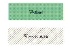
 Area Fill Patterns
|
Global Mapper Fill Patterns
|
|
Fill Pattern
|
Example
|
|
|
No Fill
|
|
|
Solid Fill
|
|
|
Backwards Diagonal Cross-Hatch
|
|
|
Cross-Hatch
|
|
|
Diagonal Cross-Hatch
|
|

|
Forward Diagonal Cross-Hatch
|
|
|
Horizontal Hatch
|
|
|
Vertical Hatch
|
|
|
Sand_Pattern
|
|
|
Intermittent_Water_Pattern
|
|
|
Salt_Pattern
|
|
|
Coral_Pattern
|
|
|
Black_Cross_Pattern
|
|
Black_Dot_Pattern
 Area Border Styles
|
Global Mapper Border Styles
|
|
Border Style
|
Example
|
|
|
Solid
|
|
|
Dash
|
|
|
Dot
|
|
|
Dash - Dot
|
|
|
Dash - Dot - Dot
|
|
|
Null
|
|

|
Railroad
|
|
|
Striped
|
|
|
Comb (Left Only)
|
|
|
Comb (Right Only)
|
|
|
Comb (Long Teeth, Left Only)
|
|
|
Comb (Long_Teeth, Right Only)
|
|
|
Comb (Widely Spaced, Left Only)
|
|
|
Comb (Widely Spaced, Right Only)
|
|
|
Comb (Long & Short Teeth, Left Only)
|
|

|
Comb (Long & Short Teeth, Right Only)
|
|
|
Comb (Double Teeth, Left Only)
|
|
|
Comb (Double Teeth, Right Only)
|
|
|
Comb (Triplet, Left Only)
|
|
|
Comb (Triplet, Right Only)
|
|
|
Rake (Narrow Spaced, Left Only)
|
|
|
Rake (Narrow Spaced, Right Only)
|
|
|
Rake (Widely Spaced, Left Only)
|
|
|
Rake (Widely Spaced, Right Only)
|
|

|
Solid with Minus Signs on Left
|
|
|
Solid with Minus Signs on Right
|
|
|
Solid with Plus Signs on Left
|
|
|
Solid with Plus Signs on Right
|
|
|
Solid with Dots on Left
|
|
|
Solid with Dots on Right
|
|
|
Solid with Ts on Left
|
|
|
Solid with Ts on Right
|
|
|
Solid with Rectangles on Left
|
|

|
Solid with Rectangles on Right
|
|
|
Solid with Squares on Left
|
|
|
Solid with Squares on Right
|
|
|
Half Circles (Tightly Spaced, Left Only)
|
|
|
Half Circles (Tightly Spaced, Right Only)
|
|
|
Half Circles (Widely Spaced, Left Only)
|
|
|
Half Circles (Widely Spaced, Right Only)
|
|
|
Solid with Diamonds on Left
|
|
|
Solid with Diamonds on Right
|
|

|
V Track (Opens Towards End of Null Line)
|
|
|
V Track (Opens Towards Start of Null Line)
|
|
|
C Track (Opens Towards End of Line)
|
|
|
C Track (Opens Towards Start of Line)
|
|
|
Arrow Track (Points Towards Start of Line)
|
|
|
Arrow Track (Points Towards End of Line)
|
|
|
V Track (Opens Towards End of Solid Line)
|
|
|
V Track (Opens Towards Start of Solid Line)
|
|
|
Solid with Xs Through Line
|
|

|
Solid with Diamonds along Line
|
|
|
Solid with Empty Diamonds along Line
|
|
|
Solid with Circles along Line
|
|
|
Solid with Empty Circles along Line
|
|
|
Solid with Arrow Pointing to Start
|
|
|
Solid with Arrow Pointing to End
|
|
|
Solid with Empty Circle at Start
|
|
|
Solid with Empty Circle at End
|
|
|
Solid with Black Edges
|
|
BUILT-IN LINE TYPES AND DRAWING STYLES
This section reviews the area, line and point styles built
into Global Mapper.
• Line Styles
♦ Line Type Features
♦ Drawing Styles
Line Styles
Upper line shows line types normal appearance. Lower line
shows how line type appears when "Display
Roads As Fat Lines When Zoomed In" option is checked
and display is zoomed in.
 Global Mapper's View --> Background Color... color
designation influences which lines can be seen. Any line whose color is the
same as the Global Mapper Backgrond Color will not be seen. Example, for a white
Background Color (RGB 255,255,255), the Processing/Closure Line will not be
visible.
Global Mapper's View --> Background Color... color
designation influences which lines can be seen. Any line whose color is the
same as the Global Mapper Backgrond Color will not be seen. Example, for a white
Background Color (RGB 255,255,255), the Processing/Closure Line will not be
visible.
|
Global Mapper Built-In Line Types
|
|
Line Type
|
Example
|
Drawing
Style
|
Line
Width
|
Line Color
|
|
|
Airport Runway
|
|
Solid
|
1
|
0,0,0
|
|
Alley or Driveway
|
|
Solid
|
1
|
128,128,128
|
|
Arterial Road
|
|
Solid
|
2
|
0,128,0
|
|
Bathymetric Contour, Intermediate
|
|
Solid
|
2
|
132,130,255
|
|
Bathymetric Contour, Major
|
|
Solid
|
3
|
132,130,255
|
|
Bathymetric Contour, Minor
|
|
Solid
|
1
|
132,130,255
|
|
Bathymetric Contour, Supplementary
|
|
Solid
|
1
|
132,130,255
|

|
City Boundary
|
|
Solid
|
1
|
0,0,0
|
|
Collector Road
|
|
Solid
|
1
|
255,128,0
|
|
Contour Line, Intermediate
|
|
Solid
|
2
|
128,64,0
|
|
Contour Line, Major
|
|
Solid
|
3
|
128,64,0
|
|
Contour Line, Minor
|
|
Solid
|
1
|
128,64,0
|
|
Contour Line, Supplementary
|
|
Solid
|
1
|
128,64,0
|
|
County Route
|
|
Solid
|
2
|
255,0,255
|
|
Deleted Line
|
|
Dash
|
1
|
192,192,192
|
|
Digitizer Tool Line
|
|
Striped
|
5
|
255,255,0
|
|
Dry Stream or River
|
|
Dot
|
1
|
0,0,211
|
|
Ferry Route
|
|
Solid
|
1
|
255,128,0
|
|
Grid Line
|
|
Solid
|
1
|
128,128,128
|
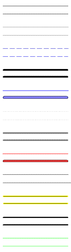
|
Grid Line - Major
|
|
Solid
|
2
|
128,128,128
|
|
Grid Line - Minor
|
|
Solid
|
1
|
128,128,128
|
|
Intermittent Stream or River
|
|
Dash
|
1
|
0,0,211
|
|
International Political
Boundary
|
|
Solid
|
6
|
0,0,0
|
|
Interstate
|
|
Solid
|
3
|
132,130,255
|
|
Invisible Boundary
|
|
Dot
|
1
|
192,192,192
|
|
Major Political Boundary
(State)
|
|
Solid
|
5
|
128,128,128
|
|
Major/US Highway
|
|
Solid
|
2
|
255,64,64
|
|
Marine Route
|
|
Solid
|
1
|
0,0,0
|
|
Measurement
|
|
Striped
|
5
|
255,255,0
|
|
Minor Political Boundary
(County)
|
|
Solid
|
4
|
0,0,0
|
|
Park Boundary
|
|
Solid
|
1
|
0,255,0
|

|
Pipeline
|
|
Dash
|
1
|
128,128,128
|
|
Powerline
|
|
Dash - Dot
|
1
|
128,128,128
|
|
Processing/Closure Line
|
|
Solid
|
2
|
255,255,255
|
|
Railroad
|
|
Railroad
|
1
|
0,0,0
|
|
Railroad, Class 1A
|
|
Railroad
|
1
|
0,0,0
|
|
Railroad, Class 1B
|
|
Railroad
|
1
|
0,0,0
|
|
Ramp
|
|
Solid
|
1
|
0,255,255
|
|
Residential Road
|
|
Solid
|
1
|
128,128,128
|
|
River, < 20 km
|
|
Solid
|
1
|
0,0,211
|
|
River, > 250 km
|
|
Solid
|
3
|
0,0,211
|
|
River, 100 - 250 km
|
|
Solid
|
3
|
0,0,211
|
|
River, 20 - 50 km
|
|
Solid
|
2
|
0,0,211
|
|
River, 50 - 100 km
|
|
Solid
|
2
|
0,0,211
|
|
River, Unknown Length
|
|
Solid
|
1
|
0,0,211
|
|
Selected Line
|
|
Dash
|
1
|
2550,0,0
|
|
Shoreline
|
|
Solid
|
1
|
0,0,0
|
|
State Highway
|
|
Solid
|
2
|
255,0,255
|
|
Stream
|
|
Solid
|
1
|
0,0,211
|
|
Tracklog
|
|
Dash
|
1
|
0,0,0
|
|
Trail
|
|
Solid
|
1
|
128,128,128
|
|
Unclassified Line Feature
|
|
Solid
|
1
|
128,128,128
|
|
Unknown Line Type
|
|
Solid
|
1
|
0,0,0
|
|
Unpaved Road
|
|
Solid
|
1
|
128,128,128
|

 Drawing Styles
Global Mapper Drawing Styles
Drawing Style Example

|
Solid
|
|
|
Dash
|
|
|
Dot
|
|
|
Dash - Dot
|
|
|
Dash - Dot - Dot
|
|
|
Null
|
|
|
Railroad
|
|
|
Striped
|
|
|
Comb (Left Only)
|
|
|
Comb (Right Only)
|
|
|
Comb (Long Teeth, Left Only)
|
|
|
Comb (Long Teeth, Right Only)
|
|
|
Comb (Widely Spaced, Left Only)
|
|
|
Comb (Widely Spaced, Right Only)
|
|
|
Comb (Long & Short Teeth, Left Only)
|
|
|
Comb (Long & Short Teeth, Right Only)
|
|
|
Comb (Double Teeth, Left Only)
|
|
|
Comb (Double Teeth, Right Only)
|
|
|
Comb (Triplet, Left Only)
|
|
|
Comb (Triplet, Right Only)
|
|
|
Rake (Narrow Spaced, Left Only)
|
|
|
Rake (Narrow Spaced, Right Only)
|
|
|
Rake (Widely Spaced, Left Only)
|
|
|
Rake (Widely Spaced, Right Only)
|
|
|
Solid with Minus Signs on Left
|
|
|
Solid with Minus Signs on Right
|
|
|
Solid with Plus Signs on Left
|
|

|
Solid with Plus Signs on Right
|
|
|
Solid with Dots on Left
|
|
|
Solid with Dots on Right
|
|
|
Solid with Ts on Left
|
|
|
Solid with Ts on Right
|
|
|
Solid with Rectangles on Left
|
|
|
Solid with Rectangles on Right
|
|
|
Solid with Squares on Left
|
|
|
Solid with Squares on Right
|
|
|
Half Circles (Tightly Spaced, Left Only)
|
|
|
Half Circles (Tightly Spaced, Right Only)
|
|
|
Half Circles (Widely Spaced, Left Only)
|
|
|
Half Circles (Widely Spaced, Right Only)
|
|
|
Solid with Diamonds on Left
|
|
|
Solid with Diamonds on Right
|
|
|
V Track (Opens Towards End of Null Line)
|
|
|
V Track (Opens Towards Start of Null Line)
|
|
|
C Track (Opens Towards End of Line)
|
|
|
C Track (Opens Towards Start of Line)
|
|
|
Arrow Track (Points Towards Start of Line)
|
|
|
Arrow Track (Points Towards End of Line)
|
|
|
V Track (Opens Towards End of Solid Line)
|
|
|
V Track (Opens Towards Start of Solid Line)
|
|
|
Solid with Xs through Line
|
|
|
Solid with Diamonds along Line
|
|
|
Solid with Empty Diamonds along Line
|
|
|
Solid with Circles along Line
|
|

|
Solid with Empty Circles along Line
|
|
|
Solid with Arrow Pointing to Start
|
|
|
Solid with Arrow Pointing to End
|
|
|
Solid with Empty Circle at Start
|
|
|
Solid with Empty Circle at End
|
|
|
Solid with Black Edges
|
|

BUILT-IN POINT TYPES AND SYMBOLS
This section reviews the area, line and point styles built
into Global Mapper.
• Point Styles
♦ Point Type Features
♦ Symbols - Basic
♦ Symbols - Geology
Point Styles
Using
the Point Styles panel users can configure what symbol will be used to display
points of a given type. In addition, the Show Labels for Points of This Type
option allows a user to turn point labels off on a
type-by-type
basis. The Custom Symbols section allows users to create new symbols from their
own bitmap and icon files which they can then use as the symbol to display for
a given type.
Global
Mapper's Point Type Features are listed in the Global Mapper Point Type
Features table. Symbols are listed in the Global Mapper Symbols table.
Global Mapper recognizes two field attributes as containing
information for the display appearence of a Point
Type. They are:
GM_TYPE=Address Label
POINT_SYMBOL=Dot - Red
 Point Type Features
|
Global Mapper Built-In Point Type Features
|
|
Point Type
|
Example
|
Symbol
|
|
|
Address Label
|
|
Dot - Red
|
|
Airport
|
|
Airport
|
|
Amusement Center
|
|
Amusement Center
|
|
Anchorage
|
|
Marina
|
|
Arch
|
|
Arch
|
|
Bank
|
|
Bank
|
|
Beacon
|
|
Dot
|
|
Boat Ramp
|
|
Boat Ramp
|
|
Bottom Conditions
|
|
Dot
|
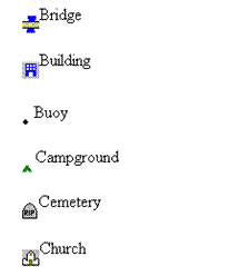


|
Bridge
|
|
Bridge
|
|
Building
|
|
School
|
|
Buoy
|
|
Dot
|
|
Campground
|
|
Campground
|
|
Cemetery
|
|
Cemetery
|
|
Church
|
|
Church
|
|
City, < 10K
|
|
Dot
|
|
City, > 10M
|
|
Dot
|
|
City, 100K - 500K
|
|
Dot
|
|
City, 10K - 50K
|
|
Dot
|
|
City, 1M - 10M
|
|
Dot
|
|
City, 500K - 1M
|
|
Dot
|
|
City, 50K - 100K
|
|
Dot
|
|
City, Population Unknown
|
|
Dot
|
|
Cliff
|
|
Cliff
|
|
Country
|
|
Dot
|
|
County
|
|
Dot
|
|
Dam
|
|
Dam
|
|
Danger
|
|
Dot
|
|
First Aid
|
|
Hospital
|
|
Geyser
|
|
Geyser
|


|
Golf Course
|
|
Golf
|
|
Hospital
|
|
Hospital
|
|
Island
|
|
Dot
|
|
Land Grant
|
|
Dot
|
|
Landmark
|
|
Dot
|
|
Library
|
|
Library
|
|
LIDAR, Building
|
|
Elevation Shaded
|
|
LIDAR, Ground Shot
|
|
Elevation Shaded
|
|
LIDAR, Power Lines
|
|
Elevation Shaded
|
|
LIDAR, Towers or Poles
|
|
Elevation Shaded
|
|
LIDAR, Unuclassified
|
|
Elevation Shaded
|
|
LIDAR, Vegetation (High)
|
|
Elevation Shaded
|
|
LIDAR, Vegetation (Low)
|
|
Elevation Shaded
|
|
LIDAR, Vegetation (Medium)
|
|
Elevation Shaded
|
|
LIDAR, Water
|
|
Elevation Shaded
|
|
Lighthouse
|
|
Lighthouse
|
|
Lodging
|
|
Lodging
|
|
Marina
|
|
Marina
|
|
Military Installation
|
|
Dot
|
|
Mine
|
|
Mine
|
|
Park
|
|
Park
|


|
Picnic Area
|
|
Picnic Area
|
|
Picture
|
|
Scenic View
|
|
Post Office
|
|
Post Office
|
|
Resturant
|
|
Resturant
|
|
Restrooms
|
|
Restrooms
|
|
Rock
|
|
Rock
|
|
School
|
|
School
|
|
Shopping
|
|
Shopping
|
|
Spot Elevation
|
|
Spot Elevation
|
|
Spot Sounding
|
|
No Symbol
|
|
Stadium
|
|
Stadium
|
|
State
|
|
Dot
|
|
Stream Origin
|
|
Stream Origin
|
|
Summit
|
|
Summit
|
|
Swimming Area
|
|
Swimming Area
|
|
Tower
|
|
Tower
|
|
Unclassified Point Feature
|
|
Dot
|
|
Unknown Point Feature
|
|
Dot
|
|
Waterfall
|
|
Waterfall
|
|
Waypoint
|
|
Dot
|
|
Weigh Station
|
|
Weigh Station
|


 Symbols
|
Global Mapper Built-In Symbols
|
|
Name
|
Symbol
|
2x Sym Details
|
|
|
Airport
|
|
|
|
Amusement Center
|
|
|
|
Arch
|
|
|
|
Auto Rental
|
|
|
|
Bank
|
|
|
|
Beacon
|
|
|
|
Big Red X
|
|
|
|
Big Yellow X
|
|
|
|
Boat Ramp
|
|
|
|
Bridge
|
|
|
|
Bullseye
|
|
|
|
Campground
|
|
|
|
Cemetry
|
|
|
|
Church
|
|
|
|
Cliff
|
|
|
|
Dam
|
|
|
|
Danger Area
|
|
|


|
Deer
|
|
|
|
Diag Crosshair - Red
|
|
|
|
Diag Crosshair - Yellow
|
|
|
|
Dot
|
|
|
|
Dot - Blue
|
|
|
|
Dot - Green
|
|
|
|
Dot - Red
|
|
|
|
Dot - White
|
|
|
|
Dot - Yellow
|
|
|
|
Elevation Shaded
|
|
|
|
Fish
|
|
|
|
Fuel
|
|
|
|
Geyser
|
|
|
|
Golf
|
|
|
|
Hospital
|
|
|
|
Library
|
|
|
|
Lighthouse
|
|
|
|
Little Blue X
|
|
|
|
Lodging
|
|
|
|
Marina
|
|
|
|
Mine
|
|
|


|
No Symbol
|
|
|
|
Park
|
|
|
|
Phone
|
|
|
|
Picnic Area
|
|
|
|
Post Office
|
|
|
|
Resturant
|
|
|
|
Restroom
|
|
|
|
Rock
|
|
|
|
Scenic View
|
|
|
|
School
|
|
|
|
Shopping
|
|
|
|
Skiing
|
|
|
|
Spot Elevation
|
|
|
|
Stadium
|
|
|
|
Stream Origin
|
|
|
|
Summit
|
|
|
|
Swimming Area
|
|
|
|
Tower
|
|
|
|
Waterfall
|
|
|
|
Weigh Station
|
|
|
|
Well
|
|
|
|
Well - Active
|
|
|
|
Well - Active at TD
|
|
|
|
Well - Dryhole
|
|
|
|
Well - Gas
|
|
|
|
Well - Injection
|
|
|
|
Well - Location
|
|
|
|
Well - Oil
|
|
|
|
Well - Oil and Gas
|
|
|
|
Well - Suspended
|
|
|
|
Wreck
|
|
|


 Symbols - Geology
|
Global Mapper Built-In Symbols
|
|
Name
|
Symbol
|
2X Sym Details
|
|
|
Geology - Arrow (Medium, Aqua)
|
|
|
|
Geology - Arrow (Medium, Black)
|
|
|
|
Geology - Arrow (Medium, Green)
|
|
|
|
Geology - Arrow (Medium, Red)
|
|
|


|
Geology - Arrow (Small, Aqua)
|
|
|
|
Geology - Arrow (Small, Black)
|
|
|
|
Geology - Arrow (Small, Green)
|
|
|
|
Geology - Arrow (Small, Red)
|
|
|
|
Geology - Cleavage (Medium, Aqua)
|
|
|
|
Geology - Cleavage (Medium, Black)
|
|
|
|
Geology - Cleavage (Medium, Green)
|
|
|
|
Geology - Cleavage (Medium, Red)
|
|
|
|
Geology - Cleavage (Small, Aqua)
|
|
|
|
Geology - Cleavage (Small, Black)
|
|
|
|
Geology - Cleavage (Small, Green)
|
|
|


|
Geology - Cleavage (Small, Red)
|
|
|
|
Geology - Dip, Bedding (Medium, Aqua)
|
|
|
|
Geology - Dip, Bedding (Medium, Black)
|
|
|
|
Geology - Dip, Bedding (Medium, Green)
|
|
|
|
Geology - Dip, Bedding (Medium, Red)
|
|
|
|
Geology - Dip, Bedding (Small, Aqua)
|
|
|
|
Geology - Dip, Bedding (Small, Black)
|
|
|
|
Geology - Dip, Bedding (Small, Green)
|
|
|
|
Geology - Dip, Bedding (Small, Red)
|
|
|
|
Geology - Dip, Overturned (Medium, Aqua)
|
|
|
|
Geology - Dip, Overturned (Medium, Black)
|
|
|


|
Geology - Dip, Overturned (Medium, Green)
|
|
|
|
Geology - Dip, Overturned (Medium, Red)
|
|
|
|
Geology - Dip, Overturned (Small, Aqua)
|
|
|
|
Geology - Dip, Overturned (Small, Black)
|
|
|
|
Geology - Dip, Overturned (Small, Green)
|
|
|
|
Geology - Dip, Overturned (Small, Red)
|
|
|
|
Geology - Foliation, Closed (Medium, Aqua)
|
|
|
|
Geology - Foliation, Closed (Medium, Black)
|
|
|
|
Geology - Foliation, Closed (Medium, Green)
|
|
|
|
Geology - Foliation, Closed (Medium, Red)
|
|
|
|
Geology - Foliation, Closed (Small, Aqua)
|
|
|


|
Geology - Foliation, Closed (Small, Black)
|
|
|
|
Geology - Foliation, Closed (Small, Green)
|
|
|
|
Geology - Foliation, Closed (Small, Red)
|
|
|
|
Geology - Foliation, Open (Medium, Aqua)
|
|
|
|
Geology - Foliation, Open (Medium, Black)
|
|
|
|
Geology - Foliation, Open (Medium, Green)
|
|
|
|
Geology - Foliation, Open (Medium, Red)
|
|
|
|
Geology - Foliation, Open (Small, Aqua)
|
|
|
|
Geology - Foliation, Open (Small, Black)
|
|
|
|
Geology - Foliation, Open (Small, Green)
|
|
|
|
Geology - Foliation, Open (Small, Red)
|
|
|


|
Geology - Horizontal Bedding (Medium, Aqua)
|
|
|
|
Geology - Horizontal Bedding (Medium, Black)
|
|
|
|
Geology - Horizontal Bedding (Medium, Green)
|
|
|
|
Geology - Horizontal Bedding (Medium, Red)
|
|
|
|
Geology - Horizontal Bedding (Small, Aqua)
|
|
|
|
Geology - Horizontal Bedding (Small, Black)
|
|
|
|
Geology - Horizontal Bedding (Small, Green)
|
|
|
|
Geology - Horizontal Bedding (Small, Red)
|
|
|
|
Geology - Joint, Closed (Medium, Aqua)
|
|
|
|
Geology - Joint, Closed (Medium, Black)
|
|
|
|
Geology - Joint, Closed (Medium, Green)
|
|
|


|
Geology - Joint, Closed (Medium, Red)
|
|
|
|
Geology - Joint, Closed (Small, Aqua)
|
|
|
|
Geology - Joint, Closed (Small, Black)
|
|
|
|
Geology - Joint, Closed (Small, Green)
|
|
|
|
Geology - Joint, Closed (Small, Red)
|
|
|
|
Geology - Joint, Open (Medium, Aqua)
|
|
|
|
Geology - Joint, Open (Medium, Black)
|
|
|
|
Geology - Joint, Open (Medium, Green)
|
|
|
|
Geology - Joint, Open (Medium, Red)
|
|
|
|
Geology - Joint, Open (Small, Aqua)
|
|
|
|
Geology - Joint, Open (Small, Black)
|
|
|


|
Geology - Joint, Open (Small, Green)
|
|
|
|
Geology - Joint, Open (Small, Red)
|
|
|
|
Geology - Vertical Bedding (Medium, Aqua)
|
|
|
|
Geology - Vertical Bedding (Medium, Black)
|
|
|
|
Geology - Vertical Bedding (Medium, Green)
|
|
|
|
Geology - Vertical Bedding (Medium, Red)
|
|
|
|
Geology - Vertical Bedding (Small, Aqua)
|
|
|
|
Geology - Vertical Bedding (Small, Black)
|
|
|
|
Geology - Vertical Bedding (Small, Green)
|
|
|
|
Geology - Vertical Bedding (Small, Red)
|
|
|
BUILT-IN AREA, LINE AND POINT TYPES
This section reviews the area, line and point styles built
into Global Mapper.
• Area Styles
♦ Area Types
♦ Area Fill Patterns
♦ Area Border Styles
• Line Styles
♦ Line Type Features
♦ Drawing Styles
• Point Styles
♦ Point Type Features
♦ Symbols - Basic
♦ Symbols - Geology
Area Styles
Using the Area Styles panel users can configure how areas of
a given type will be displayed in Global
Mapper.
Area fill, border style and color can be modified on a type-by-type basis. The
Show Labels for Areas of This Type option allows users to turn area labels off
on a type-by-type basis.
Area Types are shown in the Global Mapper Area Types table.
Tables showing the Global Mapper Fill
Patterns and Border Styles follow the Area Types table.
Global Mapper recognizes five field attributes as containing
information for the display appearence of an Area
Type. They are:
GM_TYPE= BORDER_COLOR= BORDER_WIDTH=
BORDER_STYLE= FILL_COLOR= FILL_STYLE=
The
"FILL_ALPHA=" field attribute is recognized by Global Mapper to set
an Area Type's transparency. Values for "FILL_ALPHA=" range from 0
(Transparent) to 255 (Opaque). To determine the transparency value setting
simply multiply the percentage by 255 and round off to the nearest integer
(e.g. 75% transparency 0.75 x 255 = 191.25, use 191).
As an example, the default field attributes for the
Anchorage Area Type are:
GM_TYPE=Anchorage Area BORDER_COLOR=RGB(255,0,255) BORDER_WIDTH=1
BORDER_STYLE=Comb (Right Only)
FILL_COLOR=RGB(255,0,255) FILL_STYLE=No
Fill
To
change the type's transparency to 35% the FILL_ALPHA field attribute value
should be set equal to 89 (0.35 x 255 = 89.25).
GM_TYPE=Anchorage Area
BORDER_COLOR=RGB(255,0,255)
BORDER_WIDTH=1
BORDER_STYLE=Comb (Right Only) FILL_COLOR=RGB(255,0,255) FILL_STYLE=No Fill
FILL_ALPHA=89
Area Types
 Global Mapper's View --> Background Color... color
designation influences which areas can be seen. Any area whose color is the
same as the Global Mapper Backgrond Color will not be seen. Example, for a
white Background Color (RGB 255,255,255), the Snow or Glacier Area will not be
visible.
Global Mapper's View --> Background Color... color
designation influences which areas can be seen. Any area whose color is the
same as the Global Mapper Backgrond Color will not be seen. Example, for a
white Background Color (RGB 255,255,255), the Snow or Glacier Area will not be
visible.
|
Global Mapper Built-In Area Types
|
|
Area Type
|
Example
|
Fill Pattern
|
Fill Color
|
Border
Width
|
Border
Style
|
Border
Color
|
|
|
Anchorage
Area
|
|
No Fill
|
0,0,0
|
1
|
Comb (Right Only)
|
0,0,0
|
|
City Park
|
|
Solid Fill
|
0,235,0
|
1
|
Null
|
0,0,0
|
|
Country
|
|
No Fill
|
0,0,0
|
1
|
Solid
|
0,0,0
|
|
County
|
|
No Fill
|
0,0,0
|
2
|
Solid
|
0,0,0
|
|
County
Subdivision
|
|
No Fill
|
0,0,0
|
2
|
Solid
|
128,128,128
|
|
Coverage/Quad
|
|
No Fill
|
0,0,0
|
1
|
Solid
|
0,0,0
|
|
Cropland
|
|
Solid Fill
|
183,183,0
|
1
|
Null
|
0,0,0
|

|
Dry Lakebed
|
|
Intermittent Water Pattern
|
132,130,255
|
1
|
Null
|
0,0,0
|
|
Intermittent
Lake
|
|
Intermittent Water Pattern
|
132,130,255
|
1
|
Null
|
0,0,0
|
|
Intermittent
Stream/River
|
|
Intermittent Water Pattern
|
132,130,255
|
1
|
Null
|
0,0,0
|
|
Intertidal Area
|
|
Solid Fill
|
192,240,188
|
1
|
Null
|
0,0,0
|
|
Island
|
|
No Fill
|
0,0,0
|
1
|
Solid
|
0,0,0
|
|
Isobath Area
|
|
Solid Fill
|
132,130,255
|
1
|
Null
|
0,0,0
|
|
Iso-height Area
|
|
No Fill
|
0,0,0
|
1
|
Solid
|
128,64,0
|
|
Lake, < 0.5 sq. mi.
|
|
Solid Fill
|
0,0,211
|
1
|
Null
|
0,0,0
|
|
Lake, > 500 sq. mi.
|
|
Solid Fill
|
0,0,211
|
1
|
Null
|
0,0,0
|
|
Lake, 0.5 - 1 sq. mi.
|
|
Solid Fill
|
0,0,211
|
1
|
Null
|
0,0,0
|

|
Lake, 1 - 5 sq. mi.
|
|
Solid Fill
|
0,0,211
|
1
|
Null
|
0,0,0
|
|
Lake, 10 - 30 sq. mi.
|
|
Solid Fill
|
0,0,211
|
1
|
Null
|
0,0,0
|
|
Lake, 100 - 250 sq. mi.
|
|
Solid Fill
|
0,0,211
|
1
|
Null
|
0,0,0
|
|
Lake, 250 - 500 sq. mi.
|
|
Solid Fill
|
0,0,211
|
1
|
Null
|
0,0,0
|
|
Lake, 30 - 100 sq. mi.
|
|
Solid Fill
|
0,0,211
|
1
|
Null
|
0,0,0
|
|
Lake, 5 - 10 sq. mi.
|
|
Solid Fill
|
0,0,211
|
1
|
Null
|
0,0,0
|
|
Lake, Unknown Area
|
|
Solid Fill
|
0,0,211
|
1
|
Null
|
0,0,0
|
|
Land Area
|
|
Solid Fill
|
220,212,148
|
1
|
Null
|
0,0,0
|
|
Land Grant
|
|
No Fill
|
0,0,0
|
2
|
Null
|
0,0,0
|
|
Large Metro
Area
|
|
Solid Fill
|
255,247,181
|
1
|
Null
|
0,0,0
|

|
Major National
Park
|
|
Solid Fill
|
0,235,0
|
1
|
Null
|
0,0,0
|
|
Major River
|
|
Solid Fill
|
0,0,211
|
1
|
Null
|
0,0,0
|
|
Major State
Park
|
|
Solid Fill
|
0,235,0
|
1
|
Null
|
0,0,0
|
|
Map Catalog
Layer Bounds
|
|
Diagonal
Cros-Hatch
|
255,64,64
|
1
|
Solid
|
0,0,255
|
|
Marine Info
Area
|
|
No Fill
|
255,0,255
|
1
|
Comb (Right Only)
|
255,0,0
|
|
Marine Traffic
Area
|
|
Backwards Diagonal Cross-Hatch
|
255,0,255
|
1
|
Solid
|
0,0,0
|
|
Measurement
|
|
Horizontal
Hatch
|
255,0,0
|
5
|
Striped
|
255,255,0
|
|
Metro Area
|
|
Solid Fill
|
255,247,181
|
1
|
Null
|
0,0,0
|
|
Minor River
|
|
Solid Fill
|
0,0,211
|
1
|
Null
|
0,0,0
|
|
Misc. Manmade Structure
|
|
Solid Fill
|
255,64,64
|
1
|
Null
|
0,0,0
|

|
National Park
|
|
Solid Fill
|
0,235,0
|
1
|
Null
|
0,0,0
|
|
Ocean
|
|
Solid Fill
|
0,0,211
|
1
|
Null
|
0,0,0
|
|
Orchard or
Plantation
|
|
Solid Fill
|
255,128,0
|
1
|
Null
|
0,0,0
|
|
Range Ring
|
|
No Fill
|
0,0,0
|
3
|
Solid
|
0,0,0
|
|
Reef
|
|
Coral Pattern
|
255,0,0
|
1
|
Null
|
0,0,0
|
|
Regional River
|
|
Solid Fill
|
0,0,211
|
1
|
Null
|
0,0,0
|
|
Reservation
|
|
Solid Fill
|
255,0,0
|
1
|
Null
|
0,0,0
|
|
Rock
|
|
Solid Fill
|
104,133,138
|
1
|
Null
|
0,0,0
|
|
Salt
|
|
Salt Pattern
|
192,102,192
|
1
|
Null
|
0,0,0
|
|
Sand
|
|
Sand Pattern
|
255,255,0
|
1
|
Null
|
0,0,0
|
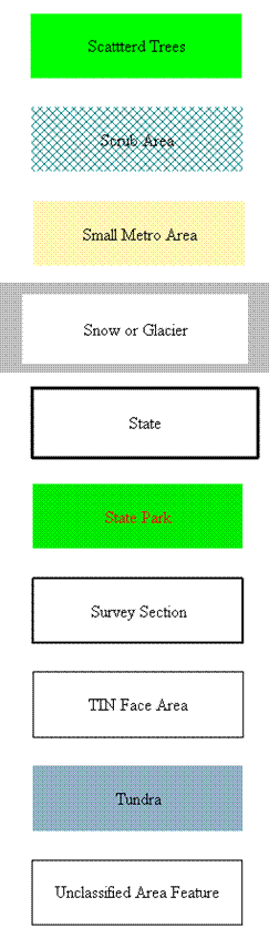
|
Scattered Trees
|
|
Solid Fill
|
0,255,0
|
1
|
Null
|
0,0,0
|
|
Scrub Area
|
|
Diagonal
Cross-Hatch
|
0,128,128
|
1
|
Null
|
0,0,0
|
|
Small Metro
Area
|
|
Solid Fill
|
255,247,181
|
1
|
Null
|
0,0,0
|
|
Snow or
Glacier
|
|
Solid Fill
|
255,255,255
|
1
|
Null
|
0,0,0
|
|
State
|
|
No Fill
|
0,0,0
|
3
|
Solid
|
0,0,0
|
|
State Park
|
|
Solid Fill
|
0,235,0
|
1
|
Null
|
0,0,0
|
|
Survey Section
|
|
No Fill
|
0,0,0
|
2
|
Solid
|
0,0,0
|
|
TIN Face Area
|
|
No Fill
|
0,0,0
|
1
|
Solid
|
0,0,0
|
|
Tundra
|
|
Solid Fill
|
145,177,196
|
1
|
Null
|
0,0,0
|
|
Unclassified
Area Feature
|
|
No Fill
|
0,0,0
|
1
|
Solid
|
0,0,0
|
|
Unknown Area
Type
|
|
No Fill
|
0,0,0
|
1
|
Solid
|
0,0,0
|
|
View Shed
Coverage Area
|
|
No Fill
|
0,0,0
|
1
|
Solid
|
0,0,0
|
|
Wetland
|
|
Solid Fill
|
125,191,167
|
1
|
Null
|
0,0,0
|
|
Wooded Area
|
|
Backwards Diagonal Cross-Hatch
|
165,145,97
|
1
|
Null
|
0,0,0
|

 Area Fill Patterns
|
Global Mapper Fill Patterns
|
|
Fill Pattern
|
Example
|
|
|
No Fill
|
|
|
Solid Fill
|
|
|
Backwards Diagonal Cross-Hatch
|
|
|
Cross-Hatch
|
|
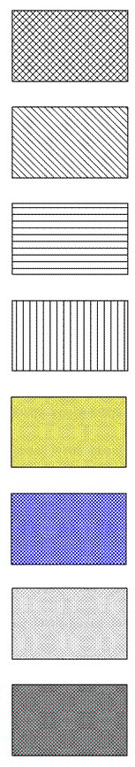
|
Diagonal Cross-Hatch
|
|
|
Forward Diagonal Cross-Hatch
|
|
|
Horizontal Hatch
|
|
|
Vertical Hatch
|
|
|
Sand_Pattern
|
|
|
Intermittent_Water_Pattern
|
|
|
Salt_Pattern
|
|
|
Coral_Pattern
|
|
|
Black_Cross_Pattern
|
|
|
Black_Dot_Pattern
|
|

 Area Border Styles
|
Global Mapper Border Styles
|
|
Border Style
|
Example
|
|
|
Solid
|
|
|
Dash
|
|
|
Dot
|
|
|
Dash - Dot
|
|
|
Dash - Dot - Dot
|
|

|
Null
|
|
|
Railroad
|
|
|
Striped
|
|
|
Comb (Left Only)
|
|
|
Comb (Right Only)
|
|
|
Comb (Long Teeth, Left Only)
|
|
|
Comb (Long_Teeth, Right Only)
|
|
|
Comb (Widely Spaced, Left Only)
|
|
|
Comb (Widely Spaced, Right Only)
|
|

|
Comb (Long & Short Teeth, Left Only)
|
|
|
Comb (Long & Short Teeth, Right Only)
|
|
|
Comb (Double Teeth, Left Only)
|
|
|
Comb (Double Teeth, Right Only)
|
|
|
Comb (Triplet, Left Only)
|
|
|
Comb (Triplet, Right Only)
|
|
|
Rake (Narrow Spaced, Left Only)
|
|
|
Rake (Narrow Spaced, Right Only)
|
|
|
Rake (Widely Spaced, Left Only)
|
|

|
Rake (Widely Spaced, Right Only)
|
|
|
Solid with Minus Signs on Left
|
|
|
Solid with Minus Signs on Right
|
|
|
Solid with Plus Signs on Left
|
|
|
Solid with Plus Signs on Right
|
|
|
Solid with Dots on Left
|
|
|
Solid with Dots on Right
|
|
|
Solid with Ts on Left
|
|
|
Solid with Ts on Right
|
|

|
Solid with Rectangles on Left
|
|
|
Solid with Rectangles on Right
|
|
|
Solid with Squares on Left
|
|
|
Solid with Squares on Right
|
|
|
Half Circles (Tightly Spaced, Left Only)
|
|
|
Half Circles (Tightly Spaced, Right Only)
|
|
|
Half Circles (Widely Spaced, Left Only)
|
|
|
Half Circles (Widely Spaced, Right Only)
|
|
|
Solid with Diamonds on Left
|
|

|
Solid with Diamonds on Right
|
|
|
V Track (Opens Towards End of Null Line)
|
|
|
V Track (Opens Towards Start of Null Line)
|
|
|
C Track (Opens Towards End of Line)
|
|
|
C Track (Opens Towards Start of Line)
|
|
|
Arrow Track (Points Towards Start of Line)
|
|
|
Arrow Track (Points Towards End of Line)
|
|
|
V Track (Opens Towards End of Solid Line)
|
|
|
V Track (Opens Towards Start of Solid Line)
|
|

|
Solid with Xs Through Line
|
|
|
Solid with Diamonds along Line
|
|
|
Solid with Empty Diamonds along Line
|
|
|
Solid with Circles along Line
|
|
|
Solid with Empty Circles along Line
|
|
|
Solid with Arrow Pointing to Start
|
|
|
Solid with Arrow Pointing to End
|
|
|
Solid with Empty Circle at Start
|
|
|
Solid with Empty Circle at End
|
|
Solid with Black Edges
 Line Styles
Using
the Line Styles panel users can configure how lines of a given type will be
displayed in Global Mapper. The line style, width, color, and label font can be
modified on a type-by-type basis. In addition, the Show Labels for Lines of
This Type option allows users to turn line labels off on a type-by-type basis.
The
Display Roads As Fat Lines When Zoomed In option allows users to turn on/off
the "fattening" of road lines when zoom in tight on them.
Global Mapper's Line Types are listed in the Global Mapper
Line Types table. Drawing Styles are listed in the
Global Mapper Drawing Styles table.
Global Mapper recognizes four field attributes as containing
information for the display appearence of a Line
Type. They are:
GM_TYPE=Airport Runway
LINE_WIDTH=1
LINE_COLOR=RGB(0,0,0) LINE_STYLE=Solid
The "LINE_STYLE=" field attribute can be set to
any one of the 60 Drawing Styles shown in the Global
Mapper Drawing Styles table. Line Types
Upper line shows line types normal
appearance. Lower line shows how line type appears when "Display
Roads As Fat Lines When Zoomed In" option is checked
and display is zoomed in.
 Global Mapper's View --> Background Color... color
designation influences which lines can be seen. Any line whose color is the
same as the Global Mapper Backgrond Color will not be seen. Example, for a
white Background Color (RGB 255,255,255), the Processing/Closure Line will not
be visible.
Global Mapper's View --> Background Color... color
designation influences which lines can be seen. Any line whose color is the
same as the Global Mapper Backgrond Color will not be seen. Example, for a
white Background Color (RGB 255,255,255), the Processing/Closure Line will not
be visible.
|
Global Mapper Built-In Line Types
|
|
Line Type
|
Example
|
Drawing
Style
|
Line
Width
|
Line Color
|
|
|
Airport Runway
|
|
Solid
|
1
|
0,0,0
|
|
Alley or Driveway
|
|
Solid
|
1
|
128,128,128
|

|
Arterial Road
|
|
Solid
|
2
|
0,128,0
|
|
Bathymetric Contour, Intermediate
|
|
Solid
|
2
|
132,130,255
|
|
Bathymetric Contour, Major
|
|
Solid
|
3
|
132,130,255
|
|
Bathymetric Contour, Minor
|
|
Solid
|
1
|
132,130,255
|
|
Bathymetric Contour, Supplementary
|
|
Solid
|
1
|
132,130,255
|
|
City Boundary
|
|
Solid
|
1
|
0,0,0
|
|
Collector Road
|
|
Solid
|
1
|
255,128,0
|
|
Contour Line, Intermediate
|
|
Solid
|
2
|
128,64,0
|
|
Contour Line, Major
|
|
Solid
|
3
|
128,64,0
|
|
Contour Line, Minor
|
|
Solid
|
1
|
128,64,0
|
|
Contour Line, Supplementary
|
|
Solid
|
1
|
128,64,0
|
|
County Route
|
|
Solid
|
2
|
255,0,255
|

|
Deleted Line
|
|
Dash
|
1
|
192,192,192
|
|
Digitizer Tool Line
|
|
Striped
|
5
|
255,255,0
|
|
Dry Stream or River
|
|
Dot
|
1
|
0,0,211
|
|
Ferry Route
|
|
Solid
|
1
|
255,128,0
|
|
Grid Line
|
|
Solid
|
1
|
128,128,128
|
|
Grid Line - Major
|
|
Solid
|
2
|
128,128,128
|
|
Grid Line - Minor
|
|
Solid
|
1
|
128,128,128
|
|
Intermittent Stream or River
|
|
Dash
|
1
|
0,0,211
|
|
International Political
Boundary
|
|
Solid
|
6
|
0,0,0
|
|
Interstate
|
|
Solid
|
3
|
132,130,255
|
|
Invisible Boundary
|
|
Dot
|
1
|
192,192,192
|
|
Major Political Boundary
(State)
|
|
Solid
|
5
|
128,128,128
|

|
Major/US Highway
|
|
Solid
|
2
|
255,64,64
|
|
Marine Route
|
|
Solid
|
1
|
0,0,0
|
|
Measurement
|
|
Striped
|
5
|
255,255,0
|
|
Minor Political Boundary
(County)
|
|
Solid
|
4
|
0,0,0
|
|
Park Boundary
|
|
Solid
|
1
|
0,255,0
|
|
Pipeline
|
|
Dash
|
1
|
128,128,128
|
|
Powerline
|
|
Dash - Dot
|
1
|
128,128,128
|
|
Processing/Closure Line
|
|
Solid
|
2
|
255,255,255
|
|
Railroad
|
|
Railroad
|
1
|
0,0,0
|
|
Railroad, Class 1A
|
|
Railroad
|
1
|
0,0,0
|
|
Railroad, Class 1B
|
|
Railroad
|
1
|
0,0,0
|
|
Ramp
|
|
Solid
|
1
|
0,255,255
|

|
Residential Road
|
|
Solid
|
1
|
128,128,128
|
|
River, < 20 km
|
|
Solid
|
1
|
0,0,211
|
|
River, > 250 km
|
|
Solid
|
3
|
0,0,211
|
|
River, 100 - 250 km
|
|
Solid
|
3
|
0,0,211
|
|
River, 20 - 50 km
|
|
Solid
|
2
|
0,0,211
|
|
River, 50 - 100 km
|
|
Solid
|
2
|
0,0,211
|
|
River, Unknown Length
|
|
Solid
|
1
|
0,0,211
|
|
Selected Line
|
|
Dash
|
1
|
2550,0,0
|
|
Shoreline
|
|
Solid
|
1
|
0,0,0
|
|
State Highway
|
|
Solid
|
2
|
255,0,255
|
|
Stream
|
|
Solid
|
1
|
0,0,211
|
|
Tracklog
|
|
Dash
|
1
|
0,0,0
|
|
Trail
|
|
Solid
|
1
|
128,128,128
|
|
Unclassified Line Feature
|
|
Solid
|
1
|
128,128,128
|
|
Unknown Line Type
|
|
Solid
|
1
|
0,0,0
|
|
Unpaved Road
|
|
Solid
|
1
|
128,128,128
|

 Drawing Styles
|
Global Mapper Drawing Styles
|
|
Drawing Style
|
Example
|
|
|
Solid
|
|
|
Dash
|
|
|
Dot
|
|
|
Dash - Dot
|
|
|
Dash - Dot - Dot
|
|
|
Null
|
|
|
Railroad
|
|
|
Striped
|
|
|
Comb (Left Only)
|
|
|
Comb (Right Only)
|
|
|
Comb (Long Teeth, Left Only)
|
|
|
Comb (Long Teeth, Right Only)
|
|
|
Comb (Widely Spaced, Left Only)
|
|
|
Comb (Widely Spaced, Right Only)
|
|
|
Comb (Long & Short Teeth, Left Only)
|
|
|
Comb (Long & Short Teeth, Right Only)
|
|
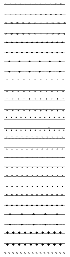
|
Comb (Double Teeth, Left Only)
|
|
|
Comb (Double Teeth, Right Only)
|
|
|
Comb (Triplet, Left Only)
|
|
|
Comb (Triplet, Right Only)
|
|
|
Rake (Narrow Spaced, Left Only)
|
|
|
Rake (Narrow Spaced, Right Only)
|
|
|
Rake (Widely Spaced, Left Only)
|
|
|
Rake (Widely Spaced, Right Only)
|
|
|
Solid with Minus Signs on Left
|
|
|
Solid with Minus Signs on Right
|
|
|
Solid with Plus Signs on Left
|
|
|
Solid with Plus Signs on Right
|
|
|
Solid with Dots on Left
|
|
|
Solid with Dots on Right
|
|
|
Solid with Ts on Left
|
|
|
Solid with Ts on Right
|
|
|
Solid with Rectangles on Left
|
|
|
Solid with Rectangles on Right
|
|
|
Solid with Squares on Left
|
|
|
Solid with Squares on Right
|
|
|
Half Circles (Tightly Spaced, Left Only)
|
|
|
Half Circles (Tightly Spaced, Right Only)
|
|
|
Half Circles (Widely Spaced, Left Only)
|
|
|
Half Circles (Widely Spaced, Right Only)
|
|
|
Solid with Diamonds on Left
|
|
|
Solid with Diamonds on Right
|
|
|
V Track (Opens Towards End of Null Line)
|
|
|
V Track (Opens Towards Start of Null Line)
|
|
|
C Track (Opens Towards End of Line)
|
|
|
C Track (Opens Towards Start of Line)
|
|
|
Arrow Track (Points Towards Start of Line)
|
|
|
Arrow Track (Points Towards End of Line)
|
|
|
V Track (Opens Towards End of Solid Line)
|
|
|
V Track (Opens Towards Start of Solid Line)
|
|
|
Solid with Xs through Line
|
|
|
Solid with Diamonds along Line
|
|
|
Solid with Empty Diamonds along Line
|
|
|
Solid with Circles along Line
|
|
|
Solid with Empty Circles along Line
|
|
|
Solid with Arrow Pointing to Start
|
|
|
Solid with Arrow Pointing to End
|
|
|
Solid with Empty Circle at Start
|
|
|
Solid with Empty Circle at End
|
|
|
Solid with Black Edges
|
|
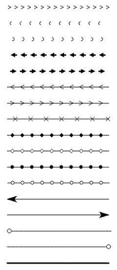 Point Styles
Using
the Point Styles panel users can configure what symbol will be used to display
points of a given type. In addition, the Show Labels for Points of This Type
option allows a user to turn point labels off on a
type-by-type
basis. The Custom Symbols section allows users to create new symbols from their
own bitmap and icon files which they can then use as the symbol to display for
a given type.
Global
Mapper's Point Type Features are listed in the Global Mapper Point Type
Features table. Symbols are listed in the Global Mapper Symbols table.
Global Mapper recognizes two field attributes as containing
information for the display appearence of a Point
Type. They are:
GM_TYPE=Address Label
POINT_SYMBOL=Dot - Red
Point Type Features
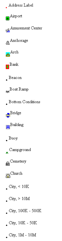
|
Global Mapper Built-In Point Type Features
|
|
Point Type
|
Example
|
Symbol
|
|
|
Address Label
|
|
Dot - Red
|
|
Airport
|
|
Airport
|
|
Amusement Center
|
|
Amusement Center
|
|
Anchorage
|
|
Marina
|
|
Arch
|
|
Arch
|
|
Bank
|
|
Bank
|
|
Beacon
|
|
Dot
|
|
Boat Ramp
|
|
Boat Ramp
|
|
Bottom Conditions
|
|
Dot
|
|
Bridge
|
|
Bridge
|
|
Building
|
|
School
|
|
Buoy
|
|
Dot
|
|
Campground
|
|
Campground
|
|
Cemetery
|
|
Cemetery
|
|
Church
|
|
Church
|
|
City, < 10K
|
|
Dot
|
|
City, > 10M
|
|
Dot
|
|
City, 100K - 500K
|
|
Dot
|
|
City, 10K - 50K
|
|
Dot
|
|
City, 1M - 10M
|
|
Dot
|
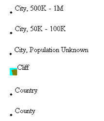


|
City, 500K - 1M
|
|
Dot
|
|
City, 50K - 100K
|
|
Dot
|
|
City, Population Unknown
|
|
Dot
|
|
Cliff
|
|
Cliff
|
|
Country
|
|
Dot
|
|
County
|
|
Dot
|
|
Dam
|
|
Dam
|
|
Danger
|
|
Dot
|
|
First Aid
|
|
Hospital
|
|
Geyser
|
|
Geyser
|
|
Golf Course
|
|
Golf
|
|
Hospital
|
|
Hospital
|
|
Island
|
|
Dot
|
|
Land Grant
|
|
Dot
|
|
Landmark
|
|
Dot
|
|
Library
|
|
Library
|
|
LIDAR, Building
|
|
Elevation Shaded
|
|
LIDAR, Ground Shot
|
|
Elevation Shaded
|
|
LIDAR, Power Lines
|
|
Elevation Shaded
|
|
LIDAR, Towers or Poles
|
|
Elevation Shaded
|
|
LIDAR, Unuclassified
|
|
Elevation Shaded
|


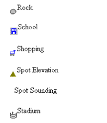
|
LIDAR, Vegetation (High)
|
|
Elevation Shaded
|
|
LIDAR, Vegetation (Low)
|
|
Elevation Shaded
|
|
LIDAR, Vegetation (Medium)
|
|
Elevation Shaded
|
|
LIDAR, Water
|
|
Elevation Shaded
|
|
Lighthouse
|
|
Lighthouse
|
|
Lodging
|
|
Lodging
|
|
Marina
|
|
Marina
|
|
Military Installation
|
|
Dot
|
|
Mine
|
|
Mine
|
|
Park
|
|
Park
|
|
Picnic Area
|
|
Picnic Area
|
|
Picture
|
|
Scenic View
|
|
Post Office
|
|
Post Office
|
|
Resturant
|
|
Resturant
|
|
Restrooms
|
|
Restrooms
|
|
Rock
|
|
Rock
|
|
School
|
|
School
|
|
Shopping
|
|
Shopping
|
|
Spot Elevation
|
|
Spot Elevation
|
|
Spot Sounding
|
|
No Symbol
|
|
Stadium
|
|
Stadium
|
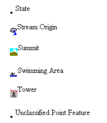
|
State
|
|
Dot
|
|
Stream Origin
|
|
Stream Origin
|
|
Summit
|
|
Summit
|
|
Swimming Area
|
|
Swimming Area
|
|
Tower
|
|
Tower
|
|
Unclassified Point Feature
|
|
Dot
|
|
Unknown Point Feature
|
|
Dot
|
|
Waterfall
|
|
Waterfall
|
|
Waypoint
|
|
Dot
|
|
Weigh Station
|
|
Weigh Station
|
|
Well
|
|
Well
|
|
Wreck
|
|
Wreck
|


 Symbols
|
Global Mapper Built-In Symbols
|
|
Name
|
Symbol
|
2x Sym Details
|
|
|
Airport
|
|
|
|
Amusement Center
|
|
|
|
Arch
|
|
|
|
Auto Rental
|
|
|
|
Bank
|
|
|
|
Beacon
|
|
|
|
Big Red X
|
|
|


|
Big Yellow X
|
|
|
|
Boat Ramp
|
|
|
|
Bridge
|
|
|
|
Bullseye
|
|
|
|
Campground
|
|
|
|
Cemetry
|
|
|
|
Church
|
|
|
|
Cliff
|
|
|
|
Dam
|
|
|
|
Danger Area
|
|
|
|
Deer
|
|
|
|
Diag Crosshair - Red
|
|
|
|
Diag Crosshair - Yellow
|
|
|
|
Dot
|
|
|
|
Dot - Blue
|
|
|
|
Dot - Green
|
|
|
|
Dot - Red
|
|
|
|
Dot - White
|
|
|
|
Dot - Yellow
|
|
|
|
Elevation Shaded
|
|
|
|
Fish
|
|
|


|
Fuel
|
|
|
|
Geyser
|
|
|
|
Golf
|
|
|
|
Hospital
|
|
|
|
Library
|
|
|
|
Lighthouse
|
|
|
|
Little Blue X
|
|
|
|
Lodging
|
|
|
|
Marina
|
|
|
|
Mine
|
|
|
|
No Symbol
|
|
|
|
Park
|
|
|
|
Phone
|
|
|
|
Picnic Area
|
|
|
|
Post Office
|
|
|
|
Resturant
|
|
|
|
Restroom
|
|
|
|
Rock
|
|
|
|
Scenic View
|
|
|
|
School
|
|
|
|
Shopping
|
|
|
|
Skiing
|
|
|
|
Spot Elevation
|
|
|
|
Stadium
|
|
|
|
Stream Origin
|
|
|
|
Summit
|
|
|
|
Swimming Area
|
|
|
|
Tower
|
|
|
|
Waterfall
|
|
|
|
Weigh Station
|
|
|
|
Well
|
|
|
|
Well - Active
|
|
|
|
Well - Active at TD
|
|
|
|
Well - Dryhole
|
|
|
|
Well - Gas
|
|
|
|
Well - Injection
|
|
|
|
Well - Location
|
|
|
|
Well - Oil
|
|
|
|
Well - Oil and Gas
|
|
|
|
Well - Suspended
|
|
|
|
Wreck
|
|
|

 Symbols - Geology


|
Global Mapper Built-In Symbols
|
|
Name
|
Symbol
|
2X Sym Details
|
|
|
Geology - Arrow (Medium, Aqua)
|
|
|
|
Geology - Arrow (Medium, Black)
|
|
|
|
Geology - Arrow (Medium, Green)
|
|
|
|
Geology - Arrow (Medium, Red)
|
|
|
|
Geology - Arrow (Small, Aqua)
|
|
|
|
Geology - Arrow (Small, Black)
|
|
|
|
Geology - Arrow (Small, Green)
|
|
|
|
Geology - Arrow (Small, Red)
|
|
|
|
Geology - Cleavage (Medium, Aqua)
|
|
|
|
Geology - Cleavage (Medium, Black)
|
|
|


|
Geology - Cleavage (Medium, Green)
|
|
|
|
Geology - Cleavage (Medium, Red)
|
|
|
|
Geology - Cleavage (Small, Aqua)
|
|
|
|
Geology - Cleavage (Small, Black)
|
|
|
|
Geology - Cleavage (Small, Green)
|
|
|
|
Geology - Cleavage (Small, Red)
|
|
|
|
Geology - Dip, Bedding (Medium, Aqua)
|
|
|
|
Geology - Dip, Bedding (Medium, Black)
|
|
|
|
Geology - Dip, Bedding (Medium, Green)
|
|
|
|
Geology - Dip, Bedding (Medium, Red)
|
|
|
|
Geology - Dip, Bedding (Small, Aqua)
|
|
|


|
Geology - Dip, Bedding (Small, Black)
|
|
|
|
Geology - Dip, Bedding (Small, Green)
|
|
|
|
Geology - Dip, Bedding (Small, Red)
|
|
|
|
Geology - Dip, Overturned (Medium, Aqua)
|
|
|
|
Geology - Dip, Overturned (Medium, Black)
|
|
|
|
Geology - Dip, Overturned (Medium, Green)
|
|
|
|
Geology - Dip, Overturned (Medium, Red)
|
|
|
|
Geology - Dip, Overturned (Small, Aqua)
|
|
|
|
Geology - Dip, Overturned (Small, Black)
|
|
|
|
Geology - Dip, Overturned (Small, Green)
|
|
|
|
Geology - Dip, Overturned (Small, Red)
|
|
|


|
Geology - Foliation, Closed (Medium, Aqua)
|
|
|
|
Geology - Foliation, Closed (Medium, Black)
|
|
|
|
Geology - Foliation, Closed (Medium, Green)
|
|
|
|
Geology - Foliation, Closed (Medium, Red)
|
|
|
|
Geology - Foliation, Closed (Small, Aqua)
|
|
|
|
Geology - Foliation, Closed (Small, Black)
|
|
|
|
Geology - Foliation, Closed (Small, Green)
|
|
|
|
Geology - Foliation, Closed (Small, Red)
|
|
|
|
Geology - Foliation, Open (Medium, Aqua)
|
|
|
|
Geology - Foliation, Open (Medium, Black)
|
|
|
|
Geology - Foliation, Open (Medium, Green)
|
|
|


|
Geology - Foliation, Open (Medium, Red)
|
|
|
|
Geology - Foliation, Open (Small, Aqua)
|
|
|
|
Geology - Foliation, Open (Small, Black)
|
|
|
|
Geology - Foliation, Open (Small, Green)
|
|
|
|
Geology - Foliation, Open (Small, Red)
|
|
|
|
Geology - Horizontal Bedding (Medium, Aqua)
|
|
|
|
Geology - Horizontal Bedding (Medium, Black)
|
|
|
|
Geology - Horizontal Bedding (Medium, Green)
|
|
|
|
Geology - Horizontal Bedding (Medium, Red)
|
|
|
|
Geology - Horizontal Bedding (Small, Aqua)
|
|
|
|
Geology - Horizontal Bedding (Small, Black)
|
|
|


|
Geology - Horizontal Bedding (Small, Green)
|
|
|
|
Geology - Horizontal Bedding (Small, Red)
|
|
|
|
Geology - Joint, Closed (Medium, Aqua)
|
|
|
|
Geology - Joint, Closed (Medium, Black)
|
|
|
|
Geology - Joint, Closed (Medium, Green)
|
|
|
|
Geology - Joint, Closed (Medium, Red)
|
|
|
|
Geology - Joint, Closed (Small, Aqua)
|
|
|
|
Geology - Joint, Closed (Small, Black)
|
|
|
|
Geology - Joint, Closed (Small, Green)
|
|
|
|
Geology - Joint, Closed (Small, Red)
|
|
|
|
Geology - Joint, Open (Medium, Aqua)
|
|
|


|
Geology - Joint, Open (Medium, Black)
|
|
|
|
Geology - Joint, Open (Medium, Green)
|
|
|
|
Geology - Joint, Open (Medium, Red)
|
|
|
|
Geology - Joint, Open (Small, Aqua)
|
|
|
|
Geology - Joint, Open (Small, Black)
|
|
|
|
Geology - Joint, Open (Small, Green)
|
|
|
|
Geology - Joint, Open (Small, Red)
|
|
|
|
Geology - Vertical Bedding (Medium, Aqua)
|
|
|
|
Geology - Vertical Bedding (Medium, Black)
|
|
|
|
Geology - Vertical Bedding (Medium, Green)
|
|
|
|
Geology - Vertical Bedding (Medium, Red)
|
|
|


|
Geology - Vertical Bedding (Small, Aqua)
|
|
|
|
Geology - Vertical Bedding (Small, Black)
|
|
|
|
Geology - Vertical Bedding (Small, Green)
|
|
|
|
Geology - Vertical Bedding (Small, Red)
|
|
|
Built-in
Datums
The
following is a list of the datums built in to Global Mapper and the
transformation parameters used to convert those datums. All parameters are
given with respect to transforming from the given datum to WGS-84.
|
Datum Name
|
EPSG Code
|
Ellipsoid Name
|
d
|
|
ADINDAN
|
6201
|
Clarke 1880
|
-1
|
|
AIN EL ABD (BAHRAIN)
|
6204
|
International 1909 (Hayford/Intl 1924)
|
-1
|
|
AIN EL ABD (SAUDI ARABIA)
|
6204
|
International 1909 (Hayford/Intl 1924)
|
-1
|
|
AMERICAN SAMOA 1962
|
6169
|
Clarke 1866
|
|
|
ARATU (BRAZIL)
|
6208
|
International 1909 (Hayford/Intl 1924)
|
-1
|
|
ARC1950
|
6209
|
Clarke 1880
|
-1
|
|
ARC1960
|
6210
|
Clarke 1880
|
-1
|
|
ASTRO B4 (SOROL ATOLL)
|
Unknown
|
International 1909 (Hayford/Intl 1924)
|
1
|
|
ASTRO BEACON
|
Unknown
|
International 1909 (Hayford/Intl 1924)
|
1
|
|
ASTRO DOS 71/4
|
Unknown
|
International 1909 (Hayford/Intl 1924)
|
-3
|
|
ASTRONOMIC STATION 1952
|
Unknown
|
International 1909 (Hayford/Intl 1924)
|
1
|
|
ATS77 (NOVA SCOTIA)
|
6122
|
ATS77
|
|
|
AUSTRALIAN GEODETIC 1966
|
6202
|
Australian National
|
|
|
AUSTRALIAN GEODETIC 1984
|
6203
|
Australian National
|
|
|
BD72 (BELGIUM 1972)
|
6313
|
International 1909 (Hayford/Intl 1924)
|
-
|
|
BEIJING 1954
|
6214
|
Krassovsky
|
|
|
BESSEL 1841 (ITALIA) [Castanea
d. F.]
|
Unknown
|
Bessel 1841
|
|
|
BESSEL 1841 (ITALIA) [Genova]
|
Unknown
|
Bessel 1841
|
|
|
BESSEL 1841 (ITALIA) [Monte
Mario]
|
Unknown
|
Bessel 1841
|
|
|
BESSEL 1841 [GREENWICH]
|
Unknown
|
Bessel 1841
|
|
|
BOGOTA OBSERVATORY
|
6218
|
International 1909 (Hayford/Intl 1924)
|
3
|
|
BUKIT RIMPAH
|
6219
|
Bessel 1841
|
-3
|
|
CAMACUPA
|
6220
|
Clarke 1880 (RGS)
|
-
|
|
CAMP AREA ASTRO
|
6715
|
International 1909 (Hayford/Intl 1924)
|
-1
|
|
CAMPO INCHAUSPE (ARGENTINA)
|
6221
|
International 1909 (Hayford/Intl 1924)
|
-1
|
|
CAPE
|
6222
|
Clarke 1880
|
-1
|
|
CARTHAGE
|
6223
|
Clarke 1880
|
-2
|
|
CHAD (WG1998)
|
Unknown
|
WGS72
|
|
|
CLARKE 1866 AUTHALIC SPHERE
|
Unknown
|
Sphere Radius 6370997 m
|
|
|
COMBANI 1950 (MAYOTTE)
|
6632
|
International 1909 (Hayford/Intl 1924)
|
-3
|
|
CORREGO ALEGRE (BRAZIL)
|
6225
|
International 1909 (Hayford/Intl 1924)
|
-2
|
|
CROATIA HDKS GRID
|
Unknown
|
Bessel 1841
|
|
|
CSJ 67 (GUYANE FRANCAISE)
|
6235
|
International 1909 (Hayford/Intl 1924)
|
-1
|
|
D-48 SLOVENIA
|
Unknown
|
Bessel 1841
|
6
|
|
DEALUL PISCULUI 1933 (ROMANIA)
|
6316
|
International 1909 (Hayford/Intl 1924)
|
1
|
|
|
X
|
DEALUL PISCULUI 1970
|
6317
|
Krassovsky
|
|
|
DEIR EZ ZOR (SYRIA)
|
6227
|
Clarke 1880 (IGN)
|
-
|
|
DUTCH (RD)
|
6289
|
Bessel 1841
|
5
|
|
EASTER ISLAND 1967
|
6719
|
International 1909 (Hayford/Intl
1924)
|
2
|
|
ED50
|
6230
|
International 1909 (Hayford/Intl
1924)
|
-
|
|
ED50 (ENGLAND)
|
6230
|
International 1909 (Hayford/Intl
1924)
|
-
|
|
ED50 (FINLAND/NORWAY)
|
6230
|
International 1909 (Hayford/Intl
1924)
|
-
|
|
ED50 (GREECE)
|
6230
|
International 1909 (Hayford/Intl
1924)
|
-
|
|
ED50 (ITALIA)
|
6230
|
International 1909 (Hayford/Intl
1924)
|
-
|
|
ED50 (MALTA)
|
6230
|
International 1909 (Hayford/Intl
1924)
|
-
|
|
ED50 (NORTH SEA)
|
6230
|
International 1909 (Hayford/Intl
1924)
|
-
|
|
ED50 (NORWAY OFFSHORE - N62)
|
6230
|
International 1909 (Hayford/Intl
1924)
|
-1
|
|
ED50 (NORWAY OFFSHORE - S62)
|
6230
|
International 1909 (Hayford/Intl
1924)
|
-
|
|
ED50 (SICILIA)
|
6230
|
International 1909 (Hayford/Intl
1924)
|
-
|
|
ED50 (SPAIN/PORTUGAL)
|
6230
|
International 1909 (Hayford/Intl
1924)
|
|
|
ED50 (TURKEY)
|
6230
|
International 1909 (Hayford/Intl
1924)
|
-
|
|
ED79
|
6668
|
International 1967
|
-
|
|
ED87
|
6231
|
International 1909 (Hayford/Intl
1924)
|
-
|
|
EGYPT 1907
|
6229
|
Helmert 1906
|
-1
|
|
EGYPT GULF OF SUEZ S-650 TL
|
6706
|
Helmert 1906
|
-1
|
|
ESTIONIA 1997
|
6180
|
GRS 1980
|
|
|
ETRF2000 - RDN
|
6326
|
GRS 1980
|
|
|
ETRS89
|
6258
|
GRS 1980
|
|
|
FD 1958 (IRAQ)
|
6132
|
Clarke 1880 (RGS)
|
-2
|
|
FINLAND/HAYFORD
|
6123
|
International 1909 (Hayford/Intl
1924)
|
-
|
|
FORT MARIGOT (ST MAARTEN)
|
6621
|
International 1909 (Hayford/Intl
1924)
|
1
|
|
GDA 94 (AUSTRALIAN GEODETIC 1994)
|
6283
|
GRS 1980
|
|
|
GDM2000 (MALAYSIA)
|
6742
|
GRS 1980
|
|
|
GGRS87 (GREECE)
|
6121
|
GRS 1980
|
-1
|
|
GOOGLE MAPS (SPHERE RADIUS 6378137)
|
Unknown
|
Sphere Radius 6378137 m
|
|
|
GRS80 ELLIPSOID
|
6326
|
GRS 1980
|
|
|
GUADELOUPE 1948
|
6622
|
International 1909 (Hayford/Intl
1924)
|
-4
|
|
GUAM 1963
|
6675
|
Clarke 1866
|
-1
|
|
HARTEBEESTHOEK 1994 (S. AFRICA)
|
6148
|
GRS 1980
|
|
|
HERAT NORTH (AFGHANISTAN)
|
6255
|
International 1909 (Hayford/Intl
1924)
|
-3
|
|
HERMANNSKOGEL
|
Unknown
|
Bessel 1841
|
6
|
|
HJORSEY 1955
|
6658
|
International 1909 (Hayford/Intl
1924)
|
-
|
|
HONG KONG 1963
|
6738
|
International 1909 (Hayford/Intl
1924)
|
-1
|
|
HONG KONG 1980
|
6611
|
International 1909 (Hayford/Intl
1924)
|
-1
|
|
HU TZU SHAN
|
6236
|
International 1909 (Hayford/Intl
1924)
|
-6
|
|
HUNGARIAN DATUM 1972
|
6237
|
GRS 1967 (Indonesia 1974)
|
|
|
IGN72 GRANDE TERRE (NEW CALEDONIA)
|
6634
|
International 1909 (Hayford/Intl
1924)
|
|
|
INDIAN (BANGLADESH)
|
Unknown
|
Everest 1830
|
2
|
|
INDIAN (MEAN VALUE)
|
Unknown
|
Everest 1830
|
1
|
|
INDIAN (NEPAL)
|
6146
|
Everest 1956
|
2
|
|
INDIAN (THAILAND)
|
Unknown
|
Everest 1830
|
2
|
|
INDIAN 1954
|
6239
|
Everest 1830
|
2
|
|
INDIAN 1960
|
6131
|
Everest 1830 (1937 Adjustment)
|
1
|
|
INDIAN 1975
|
6240
|
Everest 1830
|
2
|
|
INDONESIA 1974
|
6238
|
GRS 1967 (Indonesia 1974)
|
-
|
|
IRELAND 1965
|
Unknown
|
Modified Airy
|
5
|
|
IRELAND 1965 (1975 ADJUSTMENT)
|
Unknown
|
Modified Airy
|
4
|
|
IRENET95
|
6173
|
GRS 1980
|
|
|
ISN93 (ICELAND)
|
6659
|
GRS 1980
|
|
|
ISTS 073 ASTRO
|
Unknown
|
International 1909 (Hayford/Intl
1924)
|
2
|
|
JAD2001 (JAMAICA 2001)
|
6758
|
WGS84
|
|
|
JAD69 (JAMAICA 1969)
|
6242
|
Clarke 1866
|
|
|
JGD2000 (JAPAN)
|
6612
|
GRS 1980
|
|
|
JORDAN
|
Unknown
|
International 1909 (Hayford/Intl
1924)
|
-
|
|
KERTAU 1948
|
6245
|
Modified Everest 1948
|
-
|
|
KERTAU 1948 (MALAYSIA)
|
6245
|
Modified Everest 1948
|
-3
|
|
KKJ (FINNISH GRID)
|
6123
|
International 1909 (Hayford/Intl
1924)
|
-
|
|
KOREAN 1985
|
6162
|
Bessel 1841
|
|
|
KOREAN 1995
|
6166
|
WGS84
|
|
|
KOREAN GEODETIC DATUM (KGD)
|
6737
|
GRS 1980
|
|
|
KRASOVSKY 1940
|
Unknown
|
Krassovsky
|
|
|
LA CANOA (VENEZUELA)
|
6247
|
International 1909 (Hayford/Intl
1924)
|
-2
|
|
LE POUCE 1934 (MAURITIUS)
|
6699
|
Clarke 1880 (RGS)
|
-7
|
|
LEIGON (GHANA)
|
6250
|
Clarke 1880
|
-1
|
|
LISBON/LISBOA 1937 (DLx)
|
6207
|
International 1909 (Hayford/Intl
1924)
|
-2
|
|
LKS92 (LATVIA)
|
6661
|
GRS 1980
|
|
|
LOWRANCE
|
Unknown
|
Sphere Radius 6356752 m
|
|
|
LUREF (LUXEMBOURG)
|
Unknown
|
International 1909 (Hayford/Intl
1924)
|
|
|
LUZON (PHILIPPINES)
|
6253
|
Clarke 1866
|
-1
|
|
M'PORALOKO (GABON)
|
6266
|
Clarke 1880
|
-
|
|
MALONGO 1987
|
6259
|
International 1909 (Hayford/Intl
1924)
|
-2
|
|
MARTINIQUE 1938
|
6625
|
International 1909 (Hayford/Intl
1924)
|
1
|
|
MERCHICH (MOROCCO)
|
6261
|
Clarke 1880
|
|
|
MGI AUSTRIA
|
6312
|
Bessel 1841
|
5
|
|
MGI CROATIA/SERBIA
|
6312
|
Bessel 1841
|
5
|
|
MGI SLOVENIA
|
6312
|
Bessel 1841
|
5
|
|
MINNA (CAMEROON)
|
6263
|
Clarke 1880
|
-
|
|
MINNA (NIGERIA)
|
6263
|
Clarke 1880
|
-
|
|
MN COUNTY (ANOKA)
|
6152
|
MN County - Anoka
|
|
|
MN COUNTY (BECKER)
|
6152
|
MN County - Becker
|
|
|
MN COUNTY (BELTRAMI NORTH)
|
6152
|
MN County - Beltrami North
|
|
|
MN COUNTY (BELTRAMI SOUTH)
|
6152
|
MN County - Beltrami South
|
|
|
MN COUNTY (BENTON)
|
6152
|
MN County - Benton
|
|
|
MN COUNTY (BIG STONE)
|
6152
|
MN County - Big Stone
|
|
|
MN COUNTY (BLUE EARTH)
|
6152
|
MN County - Blue Earth
|
|
|
MN COUNTY (BROWN)
|
6152
|
MN County - Brown
|
|
|
MN COUNTY (CARLTON)
|
6152
|
MN County - Carlton
|
|
|
MN COUNTY (CARVER)
|
6152
|
MN County - Carver
|
|
|
MN COUNTY (CASS NORTH)
|
6152
|
MN County - Cass North
|
|
|
MN COUNTY (CASS SOUTH)
|
6152
|
MN County - Cass South
|
|
|
MN COUNTY (CHIPPEWA)
|
6152
|
MN County - Chippewa
|
|
|
MN COUNTY (CHISAGO)
|
6152
|
MN County - Chisago
|
|
|
MN COUNTY (COOK NORTH)
|
6152
|
MN County - Cook North
|
|
|
MN COUNTY (COOK SOUTH)
|
6152
|
MN County - Cook South
|
|
|
MN COUNTY (COTTONWOOD)
|
6152
|
MN County - Cottonwood
|
|
|
MN COUNTY (CROW WING)
|
6152
|
MN County - Crow Wing
|
|
|
MN COUNTY (DAKOTA)
|
6152
|
MN County - Dakota
|
|
|
MN COUNTY (DODGE)
|
6152
|
MN County - Dodge
|
|
|
MN COUNTY (DOUGLAS)
|
6152
|
MN County - Douglas
|
|
|
MN COUNTY (FARIBAULT)
|
6152
|
MN County - Faribault
|
|
|
MN COUNTY (FILLMORE)
|
6152
|
MN County - Fillmore
|
|
|
MN COUNTY (FREEBORN)
|
6152
|
MN County - Freeborn
|
|
|
MN COUNTY (GOODHUE)
|
6152
|
MN County - Goodhue
|
|
|
MN COUNTY (GRANT)
|
6152
|
MN County - Grant
|
|
|
MN COUNTY (HENNEPIN)
|
6152
|
MN County - Hennepin
|
|
|
MN COUNTY (HOUSTON)
|
6152
|
MN County - Houston
|
|
|
MN COUNTY (ISANTI)
|
6152
|
MN County - Isanti
|
|
|
MN COUNTY (ITASCA NORTH)
|
6152
|
MN County - Itasca North
|
|
|
MN COUNTY (ITASCA SOUTH)
|
6152
|
MN County - Itasca South
|
|
|
MN COUNTY (JACKSON)
|
6152
|
MN County - Jackson
|
|
|
MN COUNTY (KANABEC)
|
6152
|
MN County - Kanabec
|
|
|
MN COUNTY (KANDIYOHI)
|
6152
|
MN County - Kandiyohi
|
|
|
MN COUNTY (KITTSON)
|
6152
|
MN County - Kittson
|
|
|
MN COUNTY (KOOCHICHING)
|
6152
|
MN County - Koochiching
|
|
|
MN COUNTY (LAC QUI PARLE)
|
6152
|
MN County - Lac Qui Parle
|
|
|
MN COUNTY (LAKE OF THE WOODS NORTH)
|
6152
|
MN County - Lake of the Woods
North
|
|
|
MN COUNTY (LAKE OF THE WOODS SOUTH)
|
6152
|
MN County - Lake of the Woods
South
|
|
|
MN COUNTY (LE SUEUR)
|
6152
|
MN County - Le Sueur
|
|
|
MN COUNTY (LINCOLN)
|
6152
|
MN County - Lincoln
|
|
|
MN COUNTY (LYON)
|
6152
|
MN County - Lyon
|
|
|
MN COUNTY (MAHNOMEN)
|
6152
|
MN County - Mahnomen
|
|
|
MN COUNTY (MARSHALL)
|
6152
|
MN County - Marshall
|
|
|
MN COUNTY (MARTIN)
|
6152
|
MN County - Martin
|
|
|
MN COUNTY (MCLEOD)
|
6152
|
MN County - McLeod
|
|
|
MN COUNTY (MEEKER)
|
6152
|
MN County - Meeker
|
|
|
MN COUNTY (MORRISON)
|
6152
|
MN County - Morrison
|
|
|
MN COUNTY (MOWER)
|
6152
|
MN County - Mower
|
|
|
MN COUNTY (MURRAY)
|
6152
|
MN County - Murray
|
|
|
MN COUNTY (NICOLLET)
|
6152
|
MN County - Nicollet
|
|
|
MN COUNTY (NOBLES)
|
6152
|
MN County - Nobles
|
|
|
MN COUNTY (NORMAN)
|
6152
|
MN County - Norman
|
|
|
MN COUNTY (OLMSTED)
|
6152
|
MN County - Olmsted
|
|
|
MN COUNTY (OTTERTAIL)
|
6152
|
MN County - Ottertail
|
|
|
MN COUNTY (PENNINGTON)
|
6152
|
MN County - Pennington
|
|
|
MN COUNTY (PINE)
|
6152
|
MN County - Pine
|
|
|
MN COUNTY (PIPESTONE)
|
6152
|
MN County - Pipestone
|
|
|
MN COUNTY (POLK)
|
6152
|
MN County - Polk
|
|
|
MN COUNTY (POPE)
|
6152
|
MN County - Pope
|
|
|
MN COUNTY (RAMSEY)
|
6152
|
MN County - Ramsey
|
|
|
MN COUNTY (RED LAKE)
|
6152
|
MN County - Red Lake
|
|
|
MN COUNTY (REDWOOD)
|
6152
|
MN County - Redwood
|
|
|
MN COUNTY (RENVILLE)
|
6152
|
MN County - Renville
|
|
|
MN COUNTY (RICE)
|
6152
|
MN County - Rice
|
|
|
MN COUNTY (ROCK)
|
6152
|
MN County - Rock
|
|
|
MN COUNTY (ROSEAU)
|
6152
|
MN County - Roseau
|
|
|
MN COUNTY (SCOTT)
|
6152
|
MN County - Scott
|
|
|
MN COUNTY (SHERBURNE)
|
6152
|
MN County - Sherburne
|
|
|
MN COUNTY (SIBLEY)
|
6152
|
MN County - Sibley
|
|
|
MN COUNTY (ST LOUIS CENTRAL)
|
6152
|
MN County - St Louis Central
|
|
|
MN COUNTY (ST LOUIS NORTH)
|
6152
|
MN County - St Louis North
|
|
|
MN COUNTY (ST LOUIS SOUTH)
|
6152
|
MN County - St Louis South
|
|
|
MN COUNTY (STEARNS)
|
6152
|
MN County - Stearns
|
|
|
MN COUNTY (STEELE)
|
6152
|
MN County - Steele
|
|
|
MN COUNTY (STEVENS)
|
6152
|
MN County - Stevens
|
|
|
MN COUNTY (SWIFT)
|
6152
|
MN County - Swift
|
|
|
MN COUNTY (TODD)
|
6152
|
MN County - Todd
|
|
|
MN COUNTY (TRAVERSE)
|
6152
|
MN County - Traverse
|
|
|
MN COUNTY (WABASHA)
|
6152
|
MN County - Wabasha
|
|
|
MN COUNTY (WADENA)
|
6152
|
MN County - Wadena
|
|
|
MN COUNTY (WASECA)
|
6152
|
MN County - Waseca
|
|
|
MN COUNTY (WATONWAN)
|
6152
|
MN County - Watonwan
|
|
|
MN COUNTY (WINONA)
|
6152
|
MN County - Winona
|
|
|
MN COUNTY (WRIGHT)
|
6152
|
MN County - Wright
|
|
|
MN COUNTY (YELLOW MEDICINE)
|
6152
|
MN County - Yellow Medicine
|
|
|
MODIS SPHEROID (6371007.181 M)
|
Unknown
|
Sphere Radius 6371007.181 m
|
|
|
NAD27
|
6267
|
Clarke 1866
|
|
|
NAD27 (ALASKA)
|
6267
|
Clarke 1866
|
|
|
NAD27 (ALEUTIAN ISLANDS EAST)
|
6267
|
Clarke 1866
|
|
|
NAD27 (ALEUTIAN ISLANDS WEST)
|
6267
|
Clarke 1866
|
|
|
NAD27 (BAHAMAS)
|
6267
|
Clarke 1866
|
|
|
NAD27 (CANADA)
|
6267
|
Clarke 1866
|
|
|
NAD27 (CANAL ZONE)
|
6267
|
Clarke 1866
|
|
|
NAD27 (CARIBBEAN)
|
6267
|
Clarke 1866
|
|
|
NAD27 (CENTRAL AMERICA)
|
6267
|
Clarke 1866
|
|
|
NAD27 (CONUS)
|
6267
|
Clarke 1866
|
|
|
NAD27 (CUBA)
|
6267
|
Clarke 1866
|
|
|
NAD27 (GREENLAND)
|
6267
|
Clarke 1866
|
|
|
NAD27 (MEXICO)
|
6267
|
Clarke 1866
|
-
|
|
NAD27 (MICHIGAN)
|
6267
|
Clarke 1866 (Michigan)
|
|
|
NAD27 (SAN SALVADOR)
|
6267
|
Clarke 1866
|
|
|
NAD27 (YUMA PROVING GROUNDS)
|
6267
|
Clarke 1866
|
|
|
NAD83
|
6269
|
GRS 1980
|
|
|
NAD83 (ALABAMA HPGN)
|
6152
|
GRS 1980
|
|
|
NAD83 (ARIZONA HPGN)
|
6152
|
GRS 1980
|
|
|
NAD83 (ARKANSAS HPGN)
|
6152
|
GRS 1980
|
|
|
NAD83 (CALIFORNIA NORTH HPGN)
|
6152
|
GRS 1980
|
|
|
NAD83 (CALIFORNIA SOUTH HPGN)
|
6152
|
GRS 1980
|
|
|
NAD83 (COLORADO HPGN)
|
6152
|
GRS 1980
|
|
|
NAD83 (FLORIDA HPGN)
|
6152
|
GRS 1980
|
|
|
NAD83 (GEORGIA HPGN)
|
6152
|
GRS 1980
|
|
|
NAD83 (HAWAII HPGN)
|
6152
|
GRS 1980
|
|
|
NAD83 (ILLINOIS HPGN)
|
6152
|
GRS 1980
|
|
|
NAD83 (INDIANA HPGN)
|
6152
|
GRS 1980
|
|
|
NAD83 (IOWA HPGN)
|
6152
|
GRS 1980
|
|
|
NAD83 (ITRF96)
|
Unknown
|
GRS 1980
|
|
|
NAD83 (KANSAS HPGN)
|
6152
|
GRS 1980
|
|
|
NAD83 (KENTUCKY HPGN)
|
6152
|
GRS 1980
|
|
|
NAD83 (LOUISIANA HPGN)
|
6152
|
GRS 1980
|
|
|
NAD83 (MAINE HPGN)
|
6152
|
GRS 1980
|
|
|
NAD83 (MARYLAND-DELAWARE HPGN)
|
6152
|
GRS 1980
|
|
|
NAD83 (MICHIGAN HPGN)
|
6152
|
GRS 1980
|
|
|
NAD83 (MINNESOTA HPGN)
|
6152
|
GRS 1980
|
|
|
NAD83 (MISSISSIPPI HPGN)
|
6152
|
GRS 1980
|
|
|
NAD83 (MISSOURI HPGN)
|
6152
|
GRS 1980
|
|
|
NAD83 (MONTANA EAST HPGN)
|
6152
|
GRS 1980
|
|
|
NAD83 (MONTANA WEST-IDAHO HPGN)
|
6152
|
GRS 1980
|
|
|
NAD83 (NEBRASKA HPGN)
|
6152
|
GRS 1980
|
|
|
NAD83 (NEVADA HPGN)
|
6152
|
GRS 1980
|
|
|
NAD83 (NEW ENGLAND HPGN)
|
6152
|
GRS 1980
|
|
|
NAD83 (NEW JERSEY HPGN)
|
6152
|
GRS 1980
|
|
|
NAD83 (NEW MEXICO HPGN)
|
6152
|
GRS 1980
|
|
|
NAD83 (NEW YORK HPGN)
|
6152
|
GRS 1980
|
|
|
NAD83 (NORTH CAROLINA HPGN)
|
6152
|
GRS 1980
|
|
|
NAD83 (NORTH DAKOTA HPGN)
|
6152
|
GRS 1980
|
|
|
NAD83 (OHIO HPGN)
|
6152
|
GRS 1980
|
|
|
NAD83 (OKLAHOMA HPGN)
|
6152
|
GRS 1980
|
|
|
NAD83 (PENNSYLVANIA HPGN)
|
6152
|
GRS 1980
|
|
|
NAD83 (PUERTO RICO/VIRGIN ISLANDS HPGN)
|
6152
|
GRS 1980
|
|
|
NAD83 (SOUTH CAROLINA HPGN)
|
6152
|
GRS 1980
|
|
|
NAD83 (SOUTH DAKOTA HPGN)
|
6152
|
GRS 1980
|
|
|
NAD83 (TENNESSEE HPGN)
|
6152
|
GRS 1980
|
|
|
NAD83 (TEXAS EAST HPGN)
|
6152
|
GRS 1980
|
|
|
NAD83 (TEXAS WEST HPGN)
|
6152
|
GRS 1980
|
|
|
NAD83 (UTAH HPGN)
|
6152
|
GRS 1980
|
|
|
NAD83 (VIRGINIA HPGN)
|
6152
|
GRS 1980
|
|
|
NAD83 (WASHINGTON-OREGON HPGN)
|
6152
|
GRS 1980
|
|
|
NAD83 (WEST VIRGINIA HPGN)
|
6152
|
GRS 1980
|
|
|
NAD83 (WISCONSIN HPGN)
|
6152
|
GRS 1980
|
|
|
NAD83 (WYOMING HPGN)
|
6152
|
GRS 1980
|
|
|
NAD83 CSRS
|
6617
|
GRS 1980
|
|
|
NAD83 CSRS (ALBERTA)
|
6617
|
GRS 1980
|
|
|
NAD83 CSRS (BRITISH COLUMBIA)
|
6617
|
GRS 1980
|
|
|
NAD83 CSRS (NEW BRUNSWICK)
|
6617
|
GRS 1980
|
|
|
NAD83 CSRS (QUEBEC)
|
6617
|
GRS 1980
|
|
|
NAD83 CSRS (SASKATCHEWAN)
|
6617
|
GRS 1980
|
|
|
NAHRWAN (UAE)
|
6270
|
Clarke 1880 (RGS)
|
-2
|
|
NAPARIMA 1972 (TRINIDAD & TOBAGO)
|
6271
|
International 1909 (Hayford/Intl
1924)
|
|
|
NEW ISRAELI DATUM (NID)
|
6141
|
GRS 1980
|
-
|
|
NGO 1948 (GREENWICH MERIDIAN)
|
6273
|
Bessel (Modified)
|
2
|
|
NGO 1948 (OSLO MERIDIAN)
|
6817
|
Bessel (Modified)
|
2
|
|
NORTH SAHARA 1959
|
6307
|
Clarke 1880
|
-1
|
|
NORTH SAHARA 1959 (HASSI MESSAOUD)
|
6307
|
Clarke 1880
|
-1
|
|
NTF FRANCE (GREENWICH MERIDIAN)
|
6275
|
Clarke 1880 (IGN)
|
|
|
NTF FRANCE (PARIS MERIDIAN)
|
6807
|
Clarke 1880 (IGN)
|
|
|
NZGD2000
|
6167
|
GRS 1980
|
|
|
NZGD49
|
6272
|
International 1909 (Hayford/Intl
1924)
|
|
|
OBSERVATORIO 1966
|
Unknown
|
International 1909 (Hayford/Intl
1924)
|
-4
|
|
OCOTEPEQUE (COSTA RICA)
|
Unknown
|
Clarke 1866
|
2
|
|
OLD HAWAIIAN MEAN
|
6267
|
Clarke 1866
|
|
|
OLD ISRAELI DATUM (OID)
|
6281
|
Clarke 1880 (Palestine)
|
-2
|
|
OMAN
|
Unknown
|
Clarke 1880
|
-3
|
|
OSGB36 (7-PARAM TRANSFORM)
|
6277
|
Airy
|
4
|
|
OSGB36 (BEST TRANSFORM)
|
6277
|
Airy
|
|
|
OSGB36 (NTv2 GRID)
|
6277
|
Airy
|
|
|
PICO DE LAS NIEVES
|
6728
|
International 1909 (Hayford/Intl
1924)
|
-3
|
|
POINTE NOIRE 1948 (CONGO)
|
6282
|
Clarke 1880
|
-1
|
|
PORTUGESE 1973 (DATUM 73)
|
6274
|
International 1909 (Hayford/Intl
1924)
|
-2
|
|
POSGAR94 (ARGENTINA)
|
6694
|
GRS 1980
|
|
|
POTSDAM 1983 (GERMANY - FERRO)
|
6746
|
Bessel 1841
|
5
|
|
POTSDAM/DHDN (GERMANY - FERRO)
|
Unknown
|
Bessel 1841
|
|
|
POTSDAM/DHDN (GERMANY)
|
6314
|
Bessel 1841
|
|
|
PROVISIONAL SOUTH CHILEAN
|
Unknown
|
International 1909 (Hayford/Intl
1924)
|
|
|
PRS92 (PHILIPPINES)
|
6683
|
Clarke 1866
|
-1
|
|
PSAD56 (PROV. S. AMERICAN 1956)
|
6248
|
International 1909 (Hayford/Intl
1924)
|
-2
|
|
PSD93 (OMAN)
|
6134
|
Clarke 1880
|
-1
|
|
PUERTO RICO
|
6139
|
Clarke 1866
|
|
|
QND95 (QATAR)
|
6614
|
International 1909 (Hayford/Intl
1924)
|
-1
|
|
QORNOQ
|
6287
|
International 1909 (Hayford/Intl
1924)
|
1
|
|
REUNION ISLAND
|
6626
|
International 1909 (Hayford/Intl
1924)
|
|
|
REYKJAVIK 1900
|
6659
|
Danish 1876
|
-
|
|
RGF-93
|
6171
|
GRS 1980
|
|
|
RGFG95 (GUYANE)
|
6624
|
GRS 1980
|
|
|
RGM04 (MAYOTTE)
|
Unknown
|
GRS 1980
|
|
|
RGNC91-93 (NEW CALEDONIA)
|
6749
|
GRS 1980
|
|
|
RGR92 (REUNION)
|
6627
|
GRS 1980
|
|
|
RGSPM06 (ST PIERRE ET MIQUELON)
|
Unknown
|
GRS 1980
|
|
|
ROME 1940 [MONTE MARIO] (GREENWICH)
|
6265
|
International 1909 (Hayford/Intl
1924)
|
-1
|
|
ROME 1940 [MONTE MARIO] (ROME)
|
6806
|
International 1909 (Hayford/Intl
1924)
|
-1
|
|
RT90
|
6124
|
Bessel 1841
|
4
|
|
S-42 (PULKOVO 1942)
|
6284
|
Krassovsky
|
|
|
S-42 ALBANIA
|
6284
|
Krassovsky
|
|
|
S-42 AZERBAIJAN/GEORGIA
|
6284
|
Krassovsky
|
6
|
|
S-42 CZECHOSLOVAKIA
|
6284
|
Krassovsky
|
|
|
S-42 ESTONIA
|
6284
|
Krassovsky
|
|
|
S-42 GERMANY
|
6284
|
Krassovsky
|
|
|
S-42 HUNGARY
|
6284
|
Krassovsky
|
|
|
S-42 KAZAKHSTAN
|
6284
|
Krassovsky
|
|
|
S-42 LATVIA
|
6284
|
Krassovsky
|
|
|
S-42 LITHUANIA
|
6284
|
Krassovsky
|
-
|
|
S-42 POLAND
|
6284
|
Krassovsky
|
|
|
S-42 ROMANIA
|
6284
|
Krassovsky
|
|
|
S-42 RUSSIA
|
6284
|
Krassovsky
|
|
|
S-JTSK (CZECH REPUBLIC)
|
6156
|
Bessel 1841
|
5
|
|
SAO BRAZ
|
Unknown
|
International 1909 (Hayford/Intl
1924)
|
-2
|
|
SCHWARZECK (NAMIBIA)
|
6293
|
Bessel 1841
|
6
|
|
SIRGAS 2000
|
6674
|
GRS 1980
|
|
|
SOLOMON 1968 (GUX 1 ASTRO)
|
6718
|
International 1909 (Hayford/Intl
1924)
|
2
|
|
SOUTH AMERICAN 1969
|
6291
|
South America 1969
|
|
|
SOUTH AMERICAN 1969 (BRAZIL)
|
6291
|
South America 1969
|
-
|
|
SOUTHEAST BASE
|
Unknown
|
International 1909 (Hayford/Intl
1924)
|
-4
|
|
SOUTHWEST BASE
|
Unknown
|
International 1909 (Hayford/Intl
1924)
|
-1
|
|
SPHERE (RADIUS 6378137M)
|
Unknown
|
Sphere Radius 6378137 m
|
|
|
SWEREF99 (SWEDEN)
|
6619
|
GRS 1980
|
|
|
SWISS GRID (CH1903)
|
6149
|
Bessel 1841
|
6
|
|
TANANARIVE 1925 (GREENWICH)
|
6297
|
International 1909 (Hayford/Intl
1924)
|
-1
|
|
TANANARIVE 1925 (PARIS)
|
6810
|
International 1909 (Hayford/Intl
1924)
|
-1
|
|
TETE (MOZAMBIQUE)
|
6127
|
Clarke 1866
|
-1
|
|
TIMBALAI 1948
|
6298
|
Everest 1830 (1967 Definition)
|
-6
|
|
TOKYO
|
6301
|
Bessel 1841
|
-1
|
|
TRINIDAD 1903
|
6302
|
Clarke 1858
|
-
|
|
TWD67 (TAIWAN)
|
Unknown
|
GRS 1967 Modified
|
-6
|
|
VN-2000 (VIETNAM)
|
6756
|
WGS84
|
-1
|
|
WGS72
|
6322
|
WGS72
|
|
|
WGS84
|
6326
|
WGS84
|
|
|
WI COUNTY (BURNETT)
|
6152
|
WI County - Burnett
|
|
|
WI COUNTY (CHIPPEWA)
|
6152
|
WI County - Chippewa
|
|
|
WI COUNTY (DOUGLAS)
|
6152
|
WI County - Douglas
|
|
|
WI COUNTY (MARATHON)
|
6152
|
WI County - Marathon
|
|
|
WI COUNTY (SHEBOYGAN)
|
6152
|
WI County - Sheboygan
|
|
|
WI COUNTY (TAYLOR)
|
6152
|
WI County - Taylor
|
|
|
XIAN 1980 (CHINA)
|
6610
|
Xian 1980
|
|
|
YACARE (URAGUAY)
|
6309
|
International 1909 (Hayford/Intl
1924)
|
-1
|
|
ZANDERIJ (SURINAME)
|
6311
|
International 1909 (Hayford/Intl
1924)
|
-2
|
Built-in
Ellipsoids
|
Ellipsoid Name
|
Semi-Major Axis (m)
|
|
|
ATS77
|
6378135.000
|
|
|
Airy
|
6377563.396
|
|
|
Australian National
|
6378160.000
|
|
|
Bessel (Modified)
|
6377492.018
|
|
|
Bessel 1841
|
6377397.155
|
|
|
Clarke 1858
|
6378293.645
|
|
|
Clarke 1866
|
6378206.400
|
|
|
Clarke 1866 (Michigan)
|
6378450.047
|
|
|
Clarke 1880
|
6378249.145
|
|
|
Clarke 1880 (Benoit)
|
6378300.789
|
|
|
Clarke 1880 (IGN)
|
6378249.200
|
|
|
Clarke 1880 (Palestine)
|
6378300.789
|
|
|
Clarke 1880 (RGS)
|
6378249.145
|
|
|
Danish 1876
|
6377019.270
|
|
|
Everest 1830
|
6377276.345
|
|
|
Everest 1830 (1937 Adjustment)
|
6377276.345
|
|
|
Everest 1830 (1967 Definition)
|
6377298.556
|
|
|
Everest 1956
|
6377301.243
|
|
|
GRS 1967 (Indonesia 1974)
|
6378160.000
|
|
|
GRS 1967 Modified
|
6378160.000
|
|
|
GRS 1980
|
6378137.000
|
|
|
Helmert 1906
|
6378200.000
|
|
|
Hough
|
6378270.000
|
|
|
International 1909 (Hayford/Intl 1924)
|
6378388.000
|
|
|
International 1967
|
6378157.500
|
|
|
Interplanetary, Callisto
|
2408800.000
|
|
|
Interplanetary, Europa
|
1561300.000
|
|
|
Interplanetary, Ganymede
|
2634500.000
|
|
|
Interplanetary, Io
|
1826100.000
|
|
|
Interplanetary, Jupiter
|
71398000.000
|
|
|
Interplanetary, Mars 1990
|
3393400.000
|
|
|
Interplanetary, Mars 2000
|
3396190.000
|
|
|
Interplanetary, Mars 2000 Polar Sphere
|
3376200.000
|
|
|
Interplanetary, Mars 2000 Sphere
|
3396190.000
|
|
|
Interplanetary, Mercury
|
2439000.000
|
|
|
Interplanetary, Moon
|
1737400.000
|
|
|
Interplanetary, Neptune
|
24712000.000
|
|
|
Interplanetary, Pluto
|
1175000.000
|
|
|
Interplanetary, Saturn
|
60268000.000
|
|
|
Interplanetary, Titan
|
2575000.000
|
|
|
Interplanetary, Uranus
|
26200000.000
|
|
|
Interplanetary, Venus
|
6051800.000
|
|
|
Interplanetary, Venus 1985
|
6051000.000
|
|
|
Krassovsky
|
6378245.000
|
|
|
MN County - Anoka
|
6378418.941
|
|
|
MN County - Becker
|
6378586.581
|
|
|
MN County - Beltrami North
|
6378505.809
|
|
|
MN County - Beltrami South
|
6378544.823
|
|
|
MN County - Benton
|
6378490.569
|
|
|
MN County - Big Stone
|
6378470.757
|
|
|
MN County - Blue Earth
|
6378403.701
|
|
|
MN County - Brown
|
6378434.181
|
|
|
MN County - Carlton
|
6378454.907
|
|
|
MN County - Carver
|
6378400.653
|
|
|
MN County - Cass North
|
6378567.378
|
|
|
MN County - Cass South
|
6378546.957
|
|
|
MN County - Chippewa
|
6378476.853
|
|
|
MN County - Chisago
|
6378411.321
|
|
|
MN County - Cook North
|
6378647.541
|
|
|
MN County - Cook South
|
6378647.541
|
|
|
MN County - Cottonwood
|
6378514.953
|
|
|
MN County - Crow Wing
|
6378546.957
|
|
|
MN County - Dakota
|
6378421.989
|
|
|
MN County - Dodge
|
6378481.425
|
|
|
MN County - Douglas
|
6378518.001
|
|
|
MN County - Faribault
|
6378521.049
|
|
|
MN County - Fillmore
|
6378464.661
|
|
|
MN County - Freeborn
|
6378521.049
|
|
|
MN County - Goodhue
|
6378434.181
|
|
|
MN County - Grant
|
6378518.001
|
|
|
MN County - Hennepin
|
6378418.941
|
|
|
MN County - Houston
|
6378436.619
|
|
|
MN County - Isanti
|
6378411.321
|
|
|
MN County - Itasca North
|
6378574.389
|
|
|
MN County - Itasca South
|
6378574.389
|
|
|
MN County - Jackson
|
6378521.049
|
|
|
MN County - Kanabec
|
6378472.281
|
|
|
MN County - Kandiyohi
|
6378498.189
|
|
|
MN County - Kittson
|
6378449.421
|
|
|
MN County - Koochiching
|
6378525.621
|
|
|
MN County - Lac Qui Parle
|
6378476.853
|
|
|
MN County - Lake of the Woods North
|
6378466.185
|
|
|
MN County - Lake of the Woods South
|
6378496.665
|
|
|
MN County - Le Sueur
|
6378434.181
|
|
|
MN County - Lincoln
|
6378643.579
|
|
|
MN County - Lyon
|
6378559.758
|
|
|
MN County - Mahnomen
|
6378586.581
|
|
|
MN County - Marshall
|
6378441.801
|
|
|
MN County - Martin
|
6378521.049
|
|
|
MN County - McLeod
|
6378414.369
|
|
|
MN County - Meeker
|
6378498.189
|
|
|
MN County - Morrison
|
6378502.761
|
|
|
MN County - Mower
|
6378521.049
|
|
|
MN County - Murray
|
6378617.061
|
|
|
MN County - Nicollet
|
6378403.701
|
|
|
MN County - Nobles
|
6378624.681
|
|
|
MN County - Norman
|
6378468.623
|
|
|
MN County - Olmsted
|
6378481.425
|
|
|
MN County - Ottertail
|
6378525.621
|
|
|
MN County - Pennington
|
6378445.763
|
|
|
MN County - Pine
|
6378472.281
|
|
|
MN County - Pipestone
|
6378670.401
|
|
|
MN County - Polk
|
6378445.763
|
|
|
MN County - Pope
|
6378502.761
|
|
|
MN County - Ramsey
|
6378418.941
|
|
|
MN County - Red Lake
|
6378445.763
|
|
|
MN County - Redwood
|
6378438.753
|
|
|
MN County - Renville
|
6378414.369
|
|
|
MN County - Rice
|
6378434.181
|
|
|
MN County - Rock
|
6378624.681
|
|
|
MN County - Roseau
|
6378449.421
|
|
|
MN County - Scott
|
6378421.989
|
|
|
MN County - Sherburne
|
6378443.325
|
|
|
MN County - Sibley
|
6378414.369
|
|
|
MN County - St Louis Central
|
6378605.783
|
|
|
MN County - St Louis North
|
6378543.909
|
|
|
MN County - St Louis South
|
6378540.861
|
|
|
MN County - Stearns
|
6378502.761
|
|
|
MN County - Steele
|
6378481.425
|
|
|
MN County - Stevens
|
6378502.761
|
|
|
MN County - Swift
|
6378470.757
|
|
|
MN County - Todd
|
6378548.481
|
|
|
MN County - Traverse
|
6378463.746
|
|
|
MN County - Wabasha
|
6378426.561
|
|
|
MN County - Wadena
|
6378546.957
|
|
|
MN County - Waseca
|
6378481.425
|
|
|
MN County - Watonwan
|
6378514.953
|
|
|
MN County - Winona
|
6378453.688
|
|
|
MN County - Wright
|
6378443.325
|
|
|
MN County - Yellow Medicine
|
6378530.193
|
|
|
Mercury 1960
|
6378166.000
|
|
|
Modified Airy
|
6377340.189
|
|
|
Modified Everest 1948
|
6377304.063
|
|
|
Modified Mercury 1968
|
6378150.000
|
|
|
South America 1969
|
6378160.000
|
|
|
Southeast Asia
|
6378155.000
|
|
|
Sphere Radius 6356752 m
|
6356752.314
|
|
|
Sphere Radius 6370997 m
|
6370997.000
|
|
|
Sphere Radius 6371000 m
|
6371000.000
|
|
|
Sphere Radius 6371007.181 m
|
6371007.181
|
|
|
Sphere Radius 6371204 m
|
6371204.000
|
|
|
Sphere Radius 6378137 m
|
6378137.000
|
|
|
Sphere Radius 6378388 m
|
6378388.000
|
|
|
WGS66
|
6378145.000
|
|
|
WGS72
|
6378135.000
|
|
|
WGS84
|
6378137.000
|
|
|
WI County - Burnett
|
6378414.960
|
|
|
WI County - Chippewa
|
6378412.542
|
|
|
WI County - Douglas
|
6378414.930
|
|
|
WI County - Marathon
|
6378500.600
|
|
|
WI County - Sheboygan
|
6378285.480
|
|
|
WI County - Taylor
|
6378532.921
|
|
|
War Office (McCaw 1924)
|
6378300.000
|
|
|
Xian 1980
|
6378140.000
|
|